Stochastic models of epidemics

MAS316/414 Mathematical Modelling of Natural Systems Topic 2

Alex Best (a.best@shef.ac.uk)

Lecture 1: A deterministic model for epidemics

Introduction

In this topic we are going to be thinking about modelling the spread of infectious disease in some population. We will do this using a classic compartment model, where we divide the population into three types:

More detailed model structures exist, but we will focus on this initial simple model for now. We can then think about how individuals move between these three compartments to describe the dynamics of the model. Again, we will start with the simplest possible (yet biologically reasonable) structure where the only two processes are infection (Susceptible -> Infected) and recovery (Infected -> Recovered).

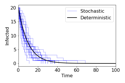
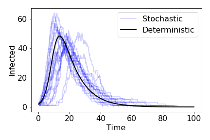
This is known as the SIR model and has formed the cornerstone of modelling infectious diseases in plant, animal and human populations since the 1920s. In general, the model is built as a set of ordinary differential equations. This is a deterministic model, where we assume the population sizes are large and that time and the variables are continuous. An important feature of this type of model is that, if we take the same parameter values and initial conditions, we will get the exact same time-course every time we run the model, and there is no randomness involved. Of course, the real world is messier than this, and we would expect a degree of inherent randomness - the precise time an infection takes place, for example. An alternative approach that captures this inherent randomness is a stochastic model. Now the same parameters and initial conditions will lead to different time-courses every time. Stochastic models can also give us more accuracy over what happens when population numbers are small and assume that events cause discrete changes in the numbers of individuals (rather than continuous changes to the density). However, their inherent randomness often makes them harder to analyse.

The deterministic model

Although our focus is to be on the stochastic implementation of a model of disease spread, it is useful for us first to get a good understanding of its deterministic counterpart. As such, let us assume that the population is large, and that both time and the population densities are continuous. We can then describe the dynamics of the model using the following ordinary differential equations,

\begin{align} &\frac{dS}{dt} = -\beta SI\label{si1}\\ &\frac{dI}{dt} = \beta SI - \gamma I\label{si2}\\ &\frac{dR}{dt} = \gamma I \end{align}

with the total population, $N=S+I+R$. Note that $dN/dt = dS/dt+dI/dt+dR/dt=0$, and so the total population stays at a constant size. This is a reasonable assumption for studying a short-term epidemic outbreak in long-lived populations. Because of this we can eliminate one variable, with $R=N-(S+I)$ and ignore the $dR/dt$ equation. We should also stress that while we will often think of these variables as numbers, they are actually densities (since they are continuous variables).

While this is a fairly simple looking system (two variables and two parameters), there is no explicit solution. However, we can explore the qualitative behaviour of the model by identifying equilibria of the system and their stability. Moreover, we can use numerical routines to simulate the possible dynamics, as we will do in the first computer lab.

Considering these equations, we can see that the only equilibrium is when $I=0$ and $S$ may take any value $<N$. We therefore seem to have a continuum of non-isolated equilibria. To assess the stability here we need to take the Jacobian of the system - a matrix made up of partial derivatives of our ODEs:

\begin{align*} J=&\left( \begin{array}{cc} \frac{\partial (dS/dt)}{\partial S} &\frac{\partial (dS/dt)}{\partial I} \\ \frac{\partial (dI/dt)}{\partial S} & \frac{\partial (dI/dt)}{\partial I} \end{array} \right)\\ =&\left( \begin{array}{cc} -\beta I & -\beta S \\ \beta I & \beta S-\gamma \end{array} \right)\\ \end{align*}

Since $I=0$ the bottom-left entry is $0$, meaning we can read the eigenvalues off as the entries on the main diagonal. We therefore have $\lambda_1=0$ and $\lambda_2=\beta S-\gamma$. The fact that one eigenvalue is 0 confirms our assessment that we have a line of non-isolated equilibria. The stability of each point now just depends on $\lambda_2$. We can see that for $S>\gamma/\beta$, the eigenvalue is positive and that point is unstable, while for $S<\gamma/\beta$, the eigenvalue is negative and that point is stable. Overall then, we expect the dynamics to eventually reach an equilibrium where $I=0$ and $S$ is some value less than $\gamma/\beta$ (but the precise value depends on the initial conditions).

This implies that in the long-run, we would expect the population to reach a point with no infected hosts i.e. the system will become disease-free. In the long-run this is often the case with emerging diseases - they will eventually burn out - but it is still important for us to know whether there can be an epidemic, when an initially small amount of infection causes a large outbreak of disease in the population (even if it eventually tends to zero).

For an epidemic to occur, we need to have $dI/dt>0$ initially. Before an outbreak, the initial densities are $S(0)\approx N,I(0)\approx0$. This gives,

\begin{equation} \frac{dI}{dt}=(\beta N-\gamma)I \end{equation}

Note that $\beta N-\gamma>0 \implies \beta N/\gamma>1$. This fraction is an important measure of how quickly a disease spreads at early points in the epidemic, and is known as the basic reproduction ratio, or $R_0$. Provided $R_0>1$, we see a classic epidemic curve, of initially exponential growth, slowing to a peak and then gradually tailing off towards 0.

Example time course of ODE model

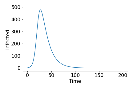
Figure 1. Example of epidemic curve from deterministic model. Paramters: $N=1000, \gamma=1/14, R_0=5$.

An extended model

We have introduced the simplest possible model for the spread of an infetcious disease, with just three possible compartments ($S$, $I$ and $R$) and only two mechanisms (infection and recovery). We have therefore built a lot of assumptions into the model, some of which are more obvious than others. Let us think about one particular extension, which is to allow immunity to wane at rate $\omega$, such that individuals who were in the recovered compartment can now return to being susceptible once again. We can then update our model as follows,

\begin{align} &\frac{dS}{dt} = -\beta SI+\omega R\\ &\frac{dI}{dt} = \beta SI - \gamma I\\ &\frac{dR}{dt} = \gamma I - \omega R. \end{align}

Notice that we still have a constant population size, meaning we can still study only the first two equations, setting $R=N-S-I$. We now have,

\begin{align} &\frac{dS}{dt} = -\beta SI+\omega (N-S-I)\\ &\frac{dI}{dt} = \beta SI - \gamma I \end{align}

We now find we have two possible equilibria. Firstly we can have $(S,I)=(N,0)$, the disease-free case. This time, however, the susceptible density takes a fixed value of $N$, because eventually everyone who was recovered will lose their immunity and return to being susceptible. The second equilibrium occurs at: $$(S,I)=\left(\frac{\gamma}{\beta},\frac{\omega\left(N-\frac{\gamma}{\beta}\right)}{\gamma+\omega}\right) $$ which after some re-arranging can be written as, $$(S,I)=\left(\frac{\gamma}{\beta},\frac{\omega\gamma}{\beta(\gamma+\omega)}(R_0-1)\right). $$

Clearly, then, the second equilibrium only exists for feasible values if $R_0>1$. It is left as a challenge for you to prove that the stability of each point depends on whether $R_0$ is larger than or less than 1.

Lecture 2: A first stochastic simulation model

We will now start thinking about how we can build a stochastic model. Recall that unlike the deterministic ODE model, we will now assume that we have discrete numbers of individuals, that there is variation in individual event rates around a mean and that the population size need not be large (in fact, large population sizes will slow us down considerably). We will use a well-known algorithm for building our stochastic model, popularly known as the Gillespie algorithm, named after the scientist who popularised the method in the 1970s (in fact, the fundamental techniques date back to the 1930s and 1940s). It is also sometimes called the direct method. This was originally designed to model chemical reactions but is equally applicable to epidemic models.

Introducing the basics

Let us start by considering an example where there is just one type of event happening. Assume we have a population of infected individuals where there is no further transmission occurring (perhaps a vaccine has rapidly removed all other susceptible individuals, or we have quarantined all infected individuals together). The only process we need to model, therefore, is recovery. The deterministic equivalent of this system would be,

\begin{equation} \frac{dI}{dt} = -\gamma I. \end{equation}

We can also think of this as a discrete event as,

\begin{align} I \xrightarrow[]{\gamma} R. \end{align}

The parameter, or rate constant, $\gamma$ has units 1/time, and is defined so that $\gamma dt$ gives the probability that a randomly chosen infected individual recovers during the time interval $[t,t+dt)$, where $dt$ is an infinitessimally small timestep. By extension, the probability that exactly one recovery happens during this interval $[t,t+dt)$ is $\gamma I(t) dt$. We would call this a first-order event, because the number of such events in some time period depends linearly on one of the variables - the number of infecteds.

Our goal is to find how many infected individuals there are at future timepoints. Let us start at $t=0$ with $I(t)=N$. Given the definitions above, our first naive attempt might be to move along at very small time intervals, $\Delta t$, and each time decide, probabalistically, whether a recovery event occurs. We could do that as follows:

  1. Choose a random number, $r$, uniformly distributed in (0,1).
  2. (a) If $r<\gamma I(t)\Delta t$, then recovery occurs. Set $I(t+\Delta t)=I(t)-1$ and update $t=t+\Delta t$.

    (b) Otherwise no recovery occurs, $I(t+\Delta t)=I(t)$ and update $t=t+\Delta t$.

Provided we set $\Delta t$ to be small enough (remember, in the definition it is assumed to be infenitessimally small), this should accurately implement the process we have described, or at least be a very good approximation of it. However, notice that if the time steps are very small, a large proportion of the time we will find that no recovery occurs and our system stays as it was. This is computationally inefficient since we spend a lot of time drawing random numbers and testing conditions only for nothing to happen. Instead, we shall try and develop a method where we only calculate one random number in between each event (and at the same time make it exact, not just a very good approximation). This links to something called 'the master equation', but here we will be focussing on how we can build a stochastic simulation algorithm.

The direct method (Gillespie algorithm)

The key to our approach is to generate random numbers that represent waiting times between events. In other words, if the current time is $t$, we are asking, "at what time $t+\tau$ will the next event occur?" We will assume $\tau$ is a continuous random variable between 0 and $\infty$. Let $f(I(t),s)ds$ be the probability that if there are $I(t)$ individuals at time $t$, the next recovery occurs in the interval $[t+s,t+s+ds)$, where $ds$ is infinitesimally small. We will call $f(I(t),s)$ the reaction probability density function. We can expand this function as meaning that there is no recovery between $t$ and $t+s$, with the recovery then ocurring in the interval $[t+s,t+s+ds)$. If we let $g(I(t),s)$ be the probability that no event occurs in the interval $[t,t+s)$, then we can write,

\begin{equation} f(I(t),s)ds=g(I(t),s)\gamma I(t+s)ds. \end{equation}

Now, since there was no recovery in the interval $[t,t+s)$ we know that $I(t+s)=I(t)$, meaning,

\begin{equation} f(I(t),s)ds=g(I(t),s)\gamma I(t)ds. \end{equation}

Let us now consider $g(I(t),s)$. For some $\sigma>0$, the probability that no recovery event happens in the interval $[t,t+\sigma+d\sigma)$ can be expressed as the product of the probability that no recovery happens in the interval $[t,t+\sigma)$ and the probability that no recovery happens in the interval $[t+\sigma,t+\sigma+d\sigma)$. This gives,

\begin{align} g(I(t),\sigma+d\sigma)&=g(I(t),\sigma)[1-\gamma I(t+\sigma)d\sigma],\\ &=g(I(t),\sigma)[1-\gamma I(t)d\sigma], \end{align}

since we know that if no recovery has happened in $[t,t+\sigma)$ it must be that $I(t+\sigma)=I(t)$. We can rearrange this to give,

\begin{equation} \frac{g(I(t),\sigma+d\sigma)-g(I(t),\sigma)}{d\sigma}=-\gamma I(t)g(I(t),\sigma). \end{equation}

If we now take the limit $d\sigma\to 0$ we can express this simply as a first-order linear differential equation,

\begin{equation} \frac{dg(I(t),\sigma)}{d\sigma}=-\gamma I(t)g(I(t),\sigma). \end{equation}

For an initial condition of $g(I(t),0)=1$ (i.e. no recovery event happens by $t=0$) and using separation of variables we obtain the solution,

\begin{equation} g(I(t),\sigma)=\exp[-\gamma I(t)\sigma]. \end{equation}

Finally we can substitute this back into our original equation for the probability that the next recovery event happens in the interval $[t+s,t+s+ds)$,

\begin{equation} f(I(t),s)ds=\exp[-\gamma I(t)s]\gamma I(t)ds. \end{equation}

We can notice that the this means the reaction probablity density function $f(I(t),s)=\exp[-\gamma I(t)s]\gamma I(t)$, which is in fact the probablity density function for the exponential distribution with mean $1/(\gamma I(t))$. In other words, the waiting times between events are exponentially distributed. We want to use this result to easily calculate waiting times, $\tau$ for the next event to occur. Let us take the function,

\begin{equation} F(\tau)=\exp[-\gamma I(t) \tau]. \end{equation}

Since $\tau$ was a random number in $[0,\infty)$, then $F(\tau)$ is a random number in the interval $[0,1]$. In fact, we can show that $F(\tau)$ is a random number uniformly distributed in the interval $[0,1]$. This is worked through below for completeness, but we will not dwell on it.

Take constants $a,b$ in the interval [0,1]. The probability that $F(\tau)$ is in the interval $(a,b)$ is the same as the probability that $\tau$ is in the interval $(F^{-1}(b),F^{-1}(a))$. This latter probability is given by the integral of $f(I(t),s)$ with respect to $s$ between $F^{-1}(b)$ and $F^{-1}(a)$. This gives,

\begin{align} \int^{F^{-1}(a)}_{F^{-1}(b)}f(I(t),s)ds &=\int^{F^{-1}(a)}_{F^{-1}(b)}\gamma I(t)\exp[-\gamma I(t)s]ds\\ &=-\int^{F^{-1}(a)}_{F^{-1}(b)}\frac{dF}{ds}ds\\ &=-F[F^{-1}(a)]+F[F^{-1}(b)]\\ &=b-a. \end{align}

We therefore know that our waiting times are exponentially distributed with mean $1/(\gamma I(t))$, and that we can find each one simply by drawing a random number uniformly distributed between 0 and 1. If we have such a random number, $r$, then we can set,

\begin{align} &r=F(\tau)=e^{-\gamma I(t)\tau}\\ \implies & \tau= \frac{1}{\gamma I(t)}\ln\left(\frac{1}{r}\right). \end{align}

Using this, we can now build our full algorithm:

  1. Set $t=0$ and $I(0)=N$.
  2. Draw a random number $r$ from the uniform distribution in $[0,1]$.
  3. Set $$\tau=\frac{1}{\gamma I(t)}\ln\left(\frac{1}{r}\right).$$
  4. (a) If $t+\tau<t_{end}$, set $t=t+\tau$ and $I(t+\tau)=I(t)-1$. If $I(t)=0$, exit. Otherwise, return to step 2.
    (b) If $t+\tau>t_{end}$, set $t=t_{end}$ and $I(t_{end})=I(t)$ and exit.

Example

We can illustrate a few steps of the algorithm with some numbers. We will populate the numbers live in the lecture. Assume a population of 20 infected individuals and that the recovery rate is $\gamma=1/10$. If we work through our algorithm we will have the following,

The figure below shows 20 trajectories from the stochastic model alongside the detrministic version. We can see that the determinsitc version is a reasonable 'average' of the stochastic runs. We can also see the variation in the stochastic runs caused by the inherent randomness.

Example of stochastic simulation
Figure 2. Example trajectories from the stochastic and deterministic versions of the recovery-only model with $\gamma=1/10$ and $I(0)=20$.

The full stochastic model

Last time we built up our first stochastic model. This was not really a true infectious disease model because the only mechanism we included was recovery. Now we shall build up our full model. Recall that the deterministic equivalent for our model is,

\begin{align} &\frac{dS}{dt} = -\beta SI\\ &\frac{dI}{dt} = \beta SI - \gamma I \end{align}

We now have two possible events,

\begin{align} S \xrightarrow[]{\beta I} I. \end{align}\begin{align} I \xrightarrow[]{\gamma} R. \end{align}

The first event occurs when a susceptible individual becomes infected. Notice that in this case the transition rate depends on the current infected density. This is a second-order event. The second event occurs, as we saw last time, when an individual recovers.

Our direct method algorithm for producing our stochastic runs is going to be very similar to what we saw last time. In particular, the time to the next event will still be exponentially distributed. However, because we now have two different types of event, the mean of the exponential distirubtion will be the inverse of the sum of all the rates. We can therefore set,

$$\rho=\beta SI+\gamma I.$$

Then if we draw a random number, $r_1$ from the uniform distribution in (0,1), the time to the next event will be,

\begin{equation} \tau = \frac{1}{\rho}\ln\left(\frac{1}{r_1}\right). \end{equation}

The second change to our algorithm is that the time we have just calculated is until the next time an event occurs, but it does not tell us which event occurs. It makes sense that the probability of one or other event happening will be proportional to their rate. Therefore, if we were to draw a second random number betweeon 0 and 1, $r_2$, then we could say,

We can now update our full algorithm:

  1. Set $t=0$, $S(0)$ and $I(0)$.
  2. Draw a random number $r_1$ from the uniform distribution in $(0,1)$.
  3. Calculate the total of all rates, $\rho$.
  4. Set $$\tau = \frac{1}{\rho}\ln\left(\frac{1}{r_1}\right).$$
  5. Check if $t+\tau<t_{end}$. If not, exit.
  6. Draw a second random number $r_2$ from the uniform distribution in $(0,1)$.
  7. (a) If $r_2\leq \gamma I/\rho$, event is recovery. Set $I(t+\tau)=I(t)-1$ and $t=t+\tau$. Return to step 2.

    (b) Otherwise event is transmission. Set $S(t+\tau)=S(t)-1$, $I(t+\tau)=I(t)+1$ and $t=t+\tau$,. Return to step 2.

An example

Again, we can illustrate a few steps of the algorithm with some numbers. Assume a population of 100 individuals, with 2 people initially infected and the rest susceptible. Assume that the recovery rate is $\gamma=1/10$ and that $R_0=2$ meaning $\beta=0.2$. We will again populate this with real numbers during the lecture.

A full time-course from 20 replicate runs is shown below.

Example of stochastic simulation

Figure 3. Example trajectories from the stochastic and deterministic versions of the recovery-only model with $\gamma=1/10$, $R_0=5$, $N=100$ and $I(0)=2$.

More complex models

This algorithm works if we have just two mechanisms at work. How will things change if we have a more complex system? For example, what about our model from the first lecture where we included waning immunity? This means we now have a third mechanism. Therefore the total rate, $\rho$ will be the sum of the three event rates. Similarly, when we check which event occurs we will need more than a single if-else statement. Most programming languages have a switch-case function, which is an effective extension of if-else statements to multpile cases. For many years python had no such functionality, and instead we would use extended if-elif-else statements. It appears that since python 3.10 was introduced, there is now a match-case statement, which is basically the same thing. Given that this is quite a recent release it is probably best to stick to if-elif-else ladders for now.

Even in the above case we still only need to keep track of two variables - susceptibles and infecteds - because we know $R=N-S-I$. If we had a model where the total population was not necessarily constant, such as the extended model seen in the first practical, then we would need to make sure we were keeping track of all three variables.