Predicting runs scored with probability distributions

The methods I covered last time only looked at win-loss probabilities. What if we wanted to predict the actual scoreline in a game? For this we'd need to understand the probability that each team scores a certain number of runs. A lot of previous work has looked at doing exactly this, especially in the context of football (soccer, for my US friends).

Runs scored as a Poisson distribution

The first attempt at predicting the number of runs scored is usually by modelling it as a Poisson process. Assuming we know the mean number of runs scored (which we can find out fairly easily), then we can find the probability of a particular number of runs, $R$, being scored in a game as,

$$P(R) = \frac{e^{-\lambda}\lambda^R}{R!}.$$

All we need is the mean number of runs, $\lambda$, to calculate this distribution (a feature of the Poisson distribution is that the mean and variance are equal). First, I will separate out home and away teams to see if there is any home advantage. In fact the mean runs scored are almost identical - home teams scored 4.59 runs on average in 2023 and away teams 4.63. The respective actual distributions for both, alongside the predictions of the Poisson model, are shown below.

In both cases, it is clear the Poission model is performing pretty poorly just by eye. Other writers have shown this to be true for baseball before, even though it seems to do an OK job for football. In particular, this model massively over-predicts the number of runs near the mean values, and under-predicts both low- and high-scoring games. This might suggest to us that we need to choose a different distribution that allows for a greater variance.

Runs scored as a negative binomial distribution

There are various ways we could move forward from the Poisson model. One next step is to use a negative binomial distribution. This is still a discrete probability distribution, but now takes in two parameters - which can be transformed into the mean and variance.

We can use a model fitting package in Python (or R, or whatever else you prefer) to fit our data to this distribution. This gives us,

	Mean	Var.
Home	4.62	10.67
Away	4.73	11.55

Again, the means are very close but slightly higher for the away team, but the variances are clearly much larger than the means. We then get the following distributions,

While these are still not perfect, in particular with some remaining under-prediction of shut-out games, it looks much better than our previous attempt. Let's work with this for now.

A full model

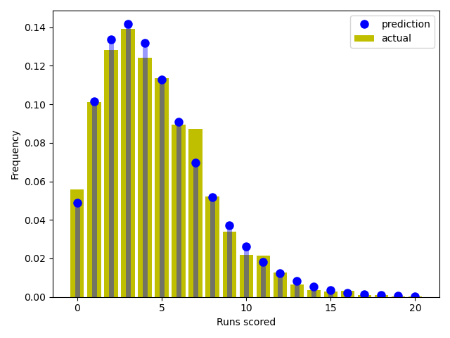
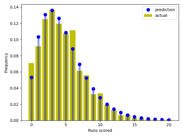
Having decided that a negative binomial distribution is a pretty good fit for runs scored in the 2023 season, we can then build up a full model. For each team, this will take in whether it was home or away (I know we've sort of decided there is no home advantage at play overall, but it might still be for some teams) and who the opponent is, and calculate the probability of scoring any number of runs in each game. I won't go into the details here, but it is a relatively straightforward thing to code in and let the software do the job for you. I borrowed much of the technical detail from other authors and took probably took some small liberties, but for now this will do us.

What can we do with this model? I have initially run the model with all the 2023 season results except the final week. We can then use our model to predict some of the results.

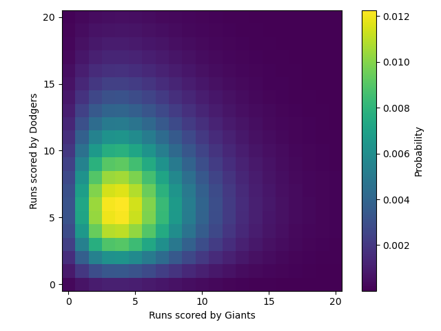
Somewhat unluckily, the Giants faced their arch-rivals the Los Angelses Dodgers in the final game of the season. Based on our model, the 'mean' runs scored would be 3.9 for the Giants and 5.3 for the Dodgers. The plot below suggests that the most likely result was a 6-4 win for the Dodgers (note that this plot allows for draws, which obviously doesn't happen in MLB, so we need to exercise a little caution interpreting this plot).

In fact, the score in that final game was a 5-2 win for the Dodgers, meaning our predictions were not far off.

Careful

In case it needs stating to anyone: I just got lucky here - remember this is all about probabilities.

In fact, let's look at all of the last round of games. How do we do with our predictions?

Game	Most likely Result	Actual Result
Cardinals vs Reds	5 - 6	4 - 3
Brewers vs Cubs	4 - 4	4 - 0
Royals vs Yankees	4 - 5	5 - 2
White Sox vs Padres	3 - 6	1 - 2
Mets vs Phillies	4 - 5	1 - 9
Rockies vs Twins	4 - 7	3 - 2
Mariners vs Rangers	5 - 5	1 - 0
Diamondbacks vs Astros	4 - 5	1 - 8
Tigers vs Guardians	4 - 4	5 - 2
Braves vs Nationals	7 - 4	9 - 10
Blue Jays vs Rays	4 - 5	8 - 12
Angels vs Athletics	6 - 4	7 - 3
Pirates vs Marlins	4 - 4	3 - 0
Giants vs Dodgers	4 - 6	2 - 5
Orioles vs Red Sox	5 - 5	1 - 6

So in fact, overall, we'd have been wise not to place too many bets based on our model (gambling is bad, kids), as of the 10 games that weren't too close to call, we only correctly predicted the winner 6 times. But again, these are probabilities, and so while we might be happy that on average we will predict the winner more times than not, there will always be games and schedules where we don't do so well.

Can we use this model to determine the best team? This is not completely straightforward, but one approach is to conduct a large number of simulated games based on the probabilities we've just calculated. Here I have set each team to play each other home and away 1500 times (meaning 87000 games per team - this seems to be about enough for things to have settled down, but ideally I'd have run more) and then ranked the by their simulated win percentage.

	Name	Simulated Pct	Actual Pct
1	Atlanta Braves	0.627	0.642
2	Los Angeles Dodgers	0.620	0.617
3	Tampa Bay Rays	0.615	0.611
4	Texas Rangers	0.592	0.556
5	Baltimore Orioles	0.580	0.623
6	Houston Astros	0.571	0.556
7	San Diego Padres	0.567	0.506
8	Minnesota Twins	0.561	0.537
9	Seattle Mariners	0.559	0.543
10	Toronto Blue Jays	0.557	0.549
11	Chicago Cubs	0.554	0.512
12	Milwaukee Brewers	0.549	0.568
13	Philadelphia Phillies	0.547	0.556
14	Boston Red Sox	0.515	0.481
15	New York Yankees	0.500	0.506
16	New York Mets	0.498	0.460
17	Arizona Diamondbacks	0.495	0.519
18	Cincinnati Reds	0.478	0.506
19	Miami Marlins	0.474	0.522
20	San Francisco Giants	0.471	0.488
21	Cleveland Guardians	0.467	0.469
22	Los Angeles Angels	0.445	0.451
23	Detroit Tigers	0.439	0.481
24	Pittsburgh Pirates	0.438	0.469
25	St. Louis Cardinals	0.434	0.438
26	Washington Nationals	0.419	0.438
27	Kansas City Royals	0.380	0.346
28	Colorado Rockies	0.373	0.364
29	Chicago White Sox	0.369	0.377
30	Oakland Athletics	0.305	0.309

This looks a little bit more like what we might have expected compared to the Elo rankings. In particular, the Braves and the Dodgers are up there at the top now, and down at the bottom we have the Athletics. Interestingly, the Texas Rangers fair much better under this framework but the Arizona Diamondbacks still appear in the bottom half of the rankings.

Summary

The methods here are a little more advanced statistically and add further detail to our predictions, namely how many runs we expect teams to score. We have seen that we may not get too many individual results correct, but overall we can draw conclusions about which are the strongest teams and on average how we might expect a specific game to play out.