14 - A model of cancer growth

14 - A model of cancer growth #

More than one in three people will develop some form of cancer during their lifetime. Given this, it is no surprise that cancer research is a hugely active field, and, relevant to this course, that there are a great many researchers interested in modelling the dynamics of cancer growth and its treatments. These models focus on a variety of important questions. We will focus on one particular model (loosely based on work by Hanhfeldt et al. (1999)).

We can model the size of a tumour by the number of cancer cells that make it up. These dynamics may actually be well represented by the logistic growth model we studied in the very first lecture (other forms, such as the Gompertz model, are often used instead, but the logistic model will do for our purposes). That is because tumours tend to be slow growing at first, then rapidly grow and finally saturate to a finite size due to resource limitations such as physical space and blood supply. Therefore, the number of cancer cells, \(c\), in a tumour may be expected to obey the dynamics,

(61)#\[\begin{equation} \frac{dc}{dt}=r_0c\left(1-\frac{c}{K}\right) \end{equation}\]

where \(r_0\) is the basic growth rate and \(K\) the carrying capacity.

An important feature of tumour growth, however, is that they can change their environment as they grow through ‘angiogenic’ factors, such that they can both stimulate and inhibit their own growth. For example, as the tumour grows it can physically create more space to grow in to, as well as secrete chemicals that encourage blood vessels to grow. On the other hand as the tumour grows it may cause damage to the blood supply. By affecting their environment in this way, cancer cells are effectively changing their own carrying capacity. Therefore, while we previously assumed a fixed carrying capacity, \(K\), it now makes sense to treat this is a dynamic variable that may grow or shrink over time depending on these angiogenic processes. The model that is proposed for these dynamics is,

(62)#\[\begin{equation} \frac{dK}{dt}=\phi c - \theta Kc^{2/3}=c\left[\phi-\theta Kc^{-1/3}\right]. \end{equation}\]

Cells stimulate the growth of blood vessels, and hence the carrying capacity, at per-capita (cell) rate \(\phi\). The inhibition rate, \(\theta\), is rather more complicated and comes from an argument about how an increasing volume of tumour will destroy local blood vessel networks.

Anaylsis#

As usual, we will proceed by finding possible equilibria, classifying their stability and drawing phase portraits.

We already know from our previous work that,

(63)#\[\begin{equation} \frac{dc}{dt}=0\implies c=0 \textrm{ or } c=K. \end{equation}\]

Substituting these values in to our second equation, we find that,

if \(c=0\), \(dK/dt\)=0 for any \(K\), and therefore there are a continuum of equilibria with no tumour but a positive carrying capacity.
if \(c=K\), \(dK/dt=0\implies c[\phi-\theta K^{2/3}]=0\). There are two different cases here. Firstly we could have \(c=K=0\) or we could have \(c=K=(\phi/\theta)^{3/2}\).

There are therefore two qualitatively different long-term solutions: either the tumour is absent (with the carrying capacity possibly at zero) or it is maintained. We should now look at the stability of these equilibria. The Jacobian of the system can be found to be,

\[\begin{align*} J=&\left( \begin{array}{cc} r\left(1-2\frac{c}{K}\right) & \frac{rc^2}{K^2}\\ \phi-\frac{2}{3}\theta Kc^{-1/3} & \theta c^{2/3} \end{array} \right) \end{align*}\]

The general case of \(c=0,K>0\) is problematic because of the lower-left entry. Of course this was already a boundary case, being a line of fixed points. We will look at this again when we draw the phase portrait. Let us first focus on the special case of \(c=K=0\) and first substitute \(c=K\) in, which leads to a number of simplifications,

Have a go

Write out the general Jacobian for this system with \(c=K\).

If we now look specifically at \(c=K=0\) we find,

\[\begin{align*} J=&\left( \begin{array}{cc} -r & r\\ \phi & 0 \end{array} \right) \end{align*}\]

Here we have \(T=-r<0\) and \(D=-r\phi<0\), meaning this equilibrium is always unstable. For the full equilibrium, since we know that \(K=(\phi/\theta)^{3/2}\), this simplifies to,

\[\begin{align*} J=&\left( \begin{array}{cc} -r & r\\ \frac{1}{3}\phi & -\phi \end{array} \right) \end{align*}\]

We therefore have, \(T=-r-\phi<0\) and \(D=\frac{2}{3}r\phi>0\), meaning the equilibrium is always stable. Together, then, these results suggest that the tumour will always grow to a fixed size and ,even with very low growth, low stimulation and high inhibition, the tumour will not be removed.

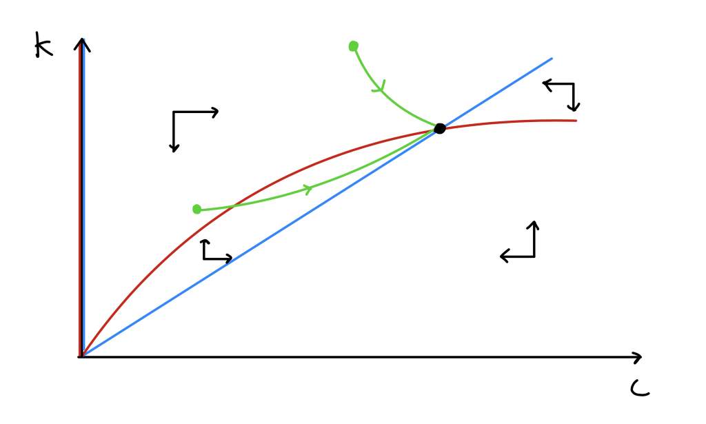
We can explore the behaviour further through plotting the phase portrait. As ever, we need to find the nullclines, determine the qualitative direction of flow, and sketch some trajectories.

Have a go

Sketch the two qualitatively different phase portraits.

Treatment#

There are many ways to treat cancer, most commonly through forms of chemotherapy and radiotherapy. Suppose we administered an anti-angiogenic drug, that reduces the carrying capacity of the tumour by limiting the blood supply. We will take a simple assumption that the drug causes a constant per-capita reduction in the carrying capacity (in reality it would be rather more complicated than this). We can model this by updating the second equation to include an additional mortality term, \(\mu\),

(64)#\[\begin{equation} \frac{dK}{dt}=\phi c - \theta Kc^{2/3}-\mu K. \end{equation}\]

After a few lines of working we can find that this changes the equilibrium values to be,

(65)#\[\begin{equation} c^*=K^*=\left(\frac{\phi-\mu}{\theta}\right)^{3/2}. \end{equation}\]

Similarly the Jacobian changes to,

\[\begin{align*} J=&\left( \begin{array}{cc} -r & r\\ \phi-\frac{2}{3}\theta K^{2/3} & -\theta K^{2/3}-\mu \end{array} \right) \end{align*}\]

and after substituting in the equilibrium yields,

\[\begin{align*} J=&\left( \begin{array}{cc} -r & r\\ \frac{1}{3}\phi+\frac{2}{3}\mu & -\phi \end{array} \right) \end{align*}\]

As before we have \(T=-r-\phi<0\), but we now have \(D=r\frac{2}{3}[\phi-\mu]\). It is now clear that if we can give a high enough treatment we can completely kill the tumour. We can also demonstrate this by re-plotting the phase portrait.

3 key points#

This model of cancer growth looks a lot like the logistic model, but with the carrying capacity also dynamic.
Without treatment a tumour will always grow to fill its space.
With treatment, the tumour can be eradicated provided the effect is strong enough.