16 - Oscillating transcription and autoregulation

Oscillating transcription

In our last model we allowed that the transcription rate, \(latex R(t)\), might depend on time but then just assumed it was constant. What if we instead assume we have an oscillating transcription rate? We will often find that we end up with expressions that are too complicated to integrate explicitly (and in that case we would probably just numerically integrate it on a computer), but if we take a sinusoidal function we can make some progress.

Let’s take the transcription function \(R(t)=r_0(1+\delta\sin(\omega t))\). This has average input \(r_0\), but varies between \(0\) and \(2r_0\), with the period depending on \(\omega\). Returning to our earlier expression, we now need to solve,

(81)\[\begin{align} M(t)&=e^{-\mu t}\int e^{\mu t}r_0\left[1+\delta\sin(\omega t)\right]dt\\ &=r_0e^{-\mu t}\left[\int e^{\mu t}dt+\delta\int e^{\mu t}\sin(\omega t)dt\right]. \end{align}\]

The first integral is identical to what we had before, so we can just copy that down again. The second may initially look a bit scary, but is actually quite a classic example of applying the method of integration by parts.

Have a go

Show that the initial solution for \(M(t)\) is given by,

(82)\[\begin{equation} r_0e^{-\mu t}\left[\frac{1}{\mu}e^{\mu t}+\frac{\delta e^{\mu t}}{\mu^2+\omega^2}(\mu\sin(\omega t)-\omega \cos(\omega t))+C\right], \end{equation}\]

where \( C\) is a constant of integration.

Click for solution

We will focus first on just finding the solution to the integral,

\[\begin{equation*} I=\int e^{\mu t}\sin(\omega t)dt, \end{equation*}\]

which we will do through integration by parts. Let \( u=e^{\mu t}\) and \( dv=\sin(\omega t)\). Then we use these to find \( du=\mu e^{\mu t}\) and \( v=-\cos(\omega t)/\omega\). The integration by parts formula is that,

\[\begin{equation*} \int udv=uv-\int vdu, \end{equation*}\]

so we have,

\[\begin{equation*} I=-\frac{1}{\omega}e^{\mu t}\cos(\omega t)+\frac{\mu}{\omega}\int e^{\mu t}\cos(\omega t)dt, \end{equation*}\]

(we should also have a constant of integration but we shall leave that out until the very end). We now have one nice term, but another tricky looking integration. Strange as it may seem, if we do integration by parts again we will make a lot of progress. Let’s take some new variables \( u=e^{\mu t}\) and \( dv=\cos(\omega t)\), meaning \( du=\mu e^{\mu t}\) and \( v=\sin(\omega t)/\omega\). This gives is an updated solution of,

\[\begin{align*} I&=-\frac{1}{\omega}e^{\mu t}\cos(\omega t)+\frac{\mu}{\omega}\left[\frac{1}{\omega}e^{\mu t}sin(\omega t)-\frac{\mu}{\omega}\int e^{\mu t}\sin(\omega t)dt\right],\\ &=\frac{1}{\omega^2}e^{\mu t}\left[-\omega\cos(\omega t)+\mu\sin(\omega t)\right]-\mu^2/\omega^2\int e^{\mu t}\sin(\omega t)dt. \end{align*}\]

This may look like we just keep making things worse! However, if you look at the remaining integral you might spot that this is actually the integral we set out to find to start with. Now that might initially seem like a problem, but it is in fact a big help. We can now write this as,

\[\begin{align*} I&=\frac{e^{\mu t}}{\omega^2}\left[-\omega\cos(\omega t)+\mu\sin(\omega t)\right]-\mu^2/\omega^2 I,\\ \implies \frac{\mu^2+\omega^2}{\omega^2}I &= \frac{e^{\mu t}}{\omega^2}\left[\mu\sin(\omega t)-\omega\cos(\omega t)\right]\\ \implies I&=\frac{e^{\mu t}}{\mu^2+\omega^2}\left[\mu\sin(\omega t)-\omega\cos(\omega t)\right]. \end{align*}\]

Now we can put this together with the solution to the more straightforward integral (and remembering our constant of integration) to find,

(83)\[\begin{equation} r_0e^{-\mu t}\left[\frac{1}{\mu}e^{\mu t}+\frac{\delta e^{\mu t}}{\mu^2+\omega^2}(\mu\sin(\omega t)-\omega \cos(\omega t))+C\right]. \end{equation}\]

We now need to complete this solution by adding in the initial condition. If we again take the initial condition that \( M(0)=0\), you should be able to show that,

\[\begin{equation*} C=\frac{\delta\omega}{\mu^2+\omega^2}-\frac{1}{\mu}, \end{equation*}\]

which leads us to the final - somewhat long - solution,

(84)\[\begin{equation} M(t)=r_0\left[\frac{1}{\mu}+\frac{\delta}{\mu^2+\omega^2}(\mu\sin(\omega t)-\omega \cos(\omega t))+\left(\frac{\delta\omega}{\mu^2+\omega^2}-\frac{1}{\mu}\right)e^{-\mu t}\right]. \end{equation}\]

As long as this is, it can readily be broken into three parts - a constant term, an oscillating term and an exponentially decaying term. After a long time we can assume the exponentially decaying term stops having much effect, meaning the solution reduces to,

(85)\[\begin{equation} M_{long-time}(t)=r_0\left[\frac{1}{\mu}+\frac{\delta}{\mu^2+\omega^2}(\mu\sin(\omega t)-\omega \cos(\omega t))\right]. \end{equation}\]

Using a few more results about trigonometric functions we can reduce this a bit further to,

(86)\[\begin{equation} M_{long-time}(t)=r_0\left[\frac{1}{\mu}+\frac{\delta}{\sqrt{\mu^2+\omega^2}}\cos(\omega t-\theta)\right], \end{equation}\]

where \( \theta=tan^{-1}(\omega/\mu)\). This then tells us that, in the long-term, the mRNA concentration oscillates around the value of \( r_0/\mu\) (the same value as in the constant case), with the same period as the inputted transcription rate (because the ‘time’ term in the cosine is \( \omega t\))), but delayed behind the input by amount \(latex \theta\). We can follow a similar approach to get an expression for \( P(t)\) as well if we wish but we won’t cover that here. A time-course of these dynamics is shown below, showing the regular fluctuations in expression.

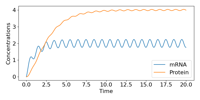
Figure: Time course of gene expression with oscillating transcription.

Modelling autoregulation

In those first examples of gene models, transcription of mRNA was due to some external resource. However, many genes encode transcription factors that directly regulate the rate of transcription of the coding gene. This produces a small feedback circuit. Representing the concentrations of mRNA and protein by \(M(t)\) and \(P(t)\) again, we can now write,

(87)\[\begin{align} \frac{dM}{dt} &= f(P) - \mu M\\ \frac{dP}{dt} &= kM - \nu P. \end{align}\]

The function \(f(P)\) must be bounded above, since transcription has a maximal rate. Furthermore \(f(P) \geq 0\) (the production rate cannot be negative!) Therefore \(f(P)\) must be non-linear, which makes the system defined by the equations above difficult, if not impossible, to solve.

To gain insight into the possible dynamics of the system, we will use qualitative analysis based around the construction of the phase portraits and linear stability analysis.

Constructing the phase portrait

Nullclines

The nullclines of the system are given by,

(88)\[\begin{align} &\frac{dM}{dt}=0 \implies M=f(P)/\mu\\ & \frac{dP}{dt}=0\implies M=\nu P/k \end{align}\]

These are both single lines/curves in the phase plane.

Equilibria

Putting the two nullcline equations equal to one another, we find a single equation for the possible equilibrium values of \(P\):

(89)\[\begin{equation} \frac{\mu\nu}{k}P^*=f(P^*). \end{equation}\]

In that case we can then find \(M^*=\nu P^*/k\) to be the corresponding equilibrium for \(M\). We can therefore focus our attention on determining the nature of any solutions for \(P^*\) for different forms of the function \(f(P)\).

Linearisation

As in previous examples, we assess stability around an equilibrium by linearisation, through looking at the Jacobian. For this model our Jacobian is,

\[\begin{align*} J=&\left( \begin{array}{cc} -\mu & f'(P^*)\\ k & -\nu \end{array} \right) \end{align*}\]

We then check the trace and determinant to assess stability:

• \(tr(J)=-\mu-\nu\)

• \(det(J)=\mu\nu-kf'(P^*)\)

The trace is always negative, limiting stability to a stable spiral or node, or an unstable saddle. Which outcome we get depends on the determinant, which in turn depends on the gradient of our transcription function at the equilibrium, \(f'(P^*)\). For the rest of this lecture and next time we will consider a few examples of what this function might look like.

Auto-repression: a negative feedback

If the protein product of a gene acts to reduce the rate of transcription, we describe it as a transcriptional repressor. The feedback circuit is described as auto-repression. In this case, \(f'(P)\leq 0\), i.e. \(f(P)\) is a decreasing function.

Recall the equation for steady state values of \(P^*\) is

(90)\[\begin{equation} \frac{\mu\nu}{k}P^*=f(P^*). \end{equation}\]

Since \(f(P)\) is strictly decreasing, this has a unique solution for \(P^*> 0\), as shown graphically below.

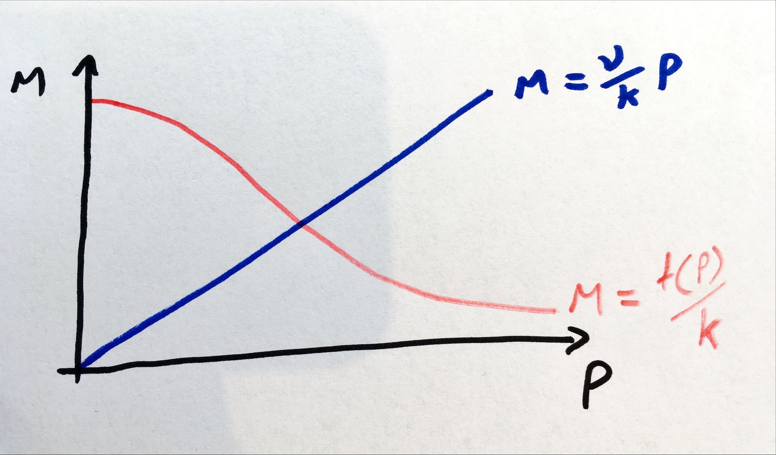
Figure: example of nullclines for auto-repression model.

We therefore have one unique equilibrium. Let us call the value of \(f'(P^*)=\phi<0\) at the equilibrium. As such we can say that \(det(J)=\mu\nu-k\phi\) is positive, meaning the equilibrium is stable. Whether the equilibrium is a node or a spiral then depends on the value of,

(91)\[\begin{align} tr^2-4det &= (\mu+\nu)^2-4\nu\mu+4k\phi\\ &=(\mu-\nu)^2+4k\phi. \end{align}\]

Firstly, we can see in the special case that \(\mu=\nu\) (the two degradation rates are equal), we just have \(4k\phi<0\), meaning we will have a stable spiral. More generally, there is a critical value,

(92)\[\begin{equation} \phi_c=-\frac{(\mu-\nu)^2}{4k}, \end{equation}\]

such that,

• if \(\phi>\phi_c\) then we have a stable node,

• if \(\phi<\phi_c\) then we have a stable spiral.

Recalling that \(\phi < 0\), we see that \(f(P)\) must be sufficiently steep at the equilibrium for it to be a spiral. The steepness of \(f(P)\) (i.e. the modulus of the derivative of \(f(P)\)) can be thought of as the “sensitivity” of the rate of transcription to changes in the protein concentration; high sensitivity means that a small change in the concentration of \(P\) results in a large change in the rate of transcription. So sensitive regulation is more likely to lead to a stable spiral.

Sketching the phase portrait

We can now sketch the phase portrait for the case of an auto-repressive gene. Note that it is easiest to draw the phase portrait with the variable \(P\) on the x-axis, and \(M\) on the y-axis.

Have a go

Using the nullclines above as a starting point, sketch the phase portrait showing how trajectories behave in this system.

Note that if the equilibrium is a spiral, then trajectories spiral in a clockwise direction. The time courses \(M(t)\) and \(P(t)\) will be damped oscillations about their equilirium values, with a peak in \(P\) following a peak in \(M\). This makes sense biologically, since mRNA acts as a template for production of protein (by translation).

3 key points

1. An autoregulatory gene network means transcription of mRNA is controlled by the concentration of protein.

2. An auto-repressive gene can be modelled by the transcription being a decreasing function of protein concentration.

3. An auto-repressive gene has a single equilibrium that can either be a stable node or spiral, depending on the model parameters.