7 - Vaccination and disease in the wild#
Vaccination#
Suppose we want to prevent a disease spreading through a vaccination programme. What proportion, \(p\), of the population do we need to vaccinate to succeed? If our vaccine works perfectly then the pre-infection density of susceptibles reduces from \(N\) to \(N(1-p)\). Recall that for the disease to die out we want \(R_0=\beta N/(\gamma+\mu)<1\). After vaccination this becomes,
Note that not all of the population needs to be vaccinated - just enough to prevent the disease from spreading freely. This is important as there may be certain groups, those undergoing medical treatment, for example, who cannot be vaccinated. This population-wide protection created by significant vaccination is called herd immunity. The higher the \(R_0\) of the disease, the greater proportion of the population that needs to be vaccinated.
Disease in the wild#
We have so far been focussing on the spread of infectious diseases through human populations. However, infectious diseases are also extremely important to the dynamics of many animal and plant populations (for example, Foot and Mouth, Bovine TB, Wheat Rust, etc.). We should therefore extend our models to consider these cases. There are three important changes we should make to the SIR model to reflect diseases in wildlife (or farmed) populations:
We shall now assume that there is no immunity (in fact, most vertebrate populations do have some immune memory, but for generality we shall neglect this). Hosts can still recover from infection, but they will simply become susceptible once again.
We can no longer reasonably assume that births and deaths are in equilibrium.
We should include the fact that disease causes significant damage to hosts (something we have so far ignored). In particular, we shall assume that infected hosts suffer an additional mortality, or {\em virulence} at rate \(\alpha\).
Our new SIS model will then be given by,
Prior to European settlement, there were no rabbits in Australia. Initially bred for food, their numbers stayed low until a small number of rabbits were released for hunting purposes on an estate. Within 10 years rabbit numbers were well in to the millions. During this initial growth period, we might actually suppose that our very first population growth model provided a good approximation of rabbit dynamics,
predicting exponential growth for \(b>d\) (births greater than deaths).
A number of control strategies were attempted through the late 19th- and early 20th-centuries targeting rabbits, from shooting to the rabbit-proof fence. In 1950, the myxoma virus was deliberately released in to the rabbit population. From a modelling perspective, the effect of this is to transform the system to the SIS model given above, that is,
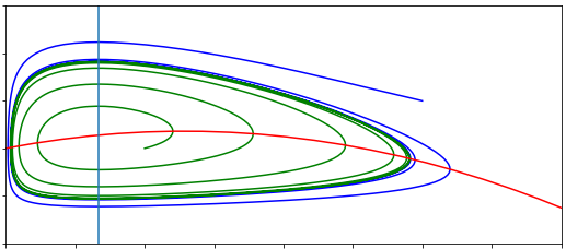
Our question is, will the introduction of the disease successfully control rabbit numbers? Initially we had exponential growth. What we then need to know is whether introducing the disease can limit this. What are the equilibria of this model? There is a trivial equilibrium at \((S,I)=(0,0)\). Also, if \(I=0\) then we return to exponential growth when \(b>d\). But there is also an endemic equilibrium, at,
To determine whether this equilibrium is stable, and so whether the disease can indeed control the rabbit population to this equilibrium level, we need to look at the Jacobian.
Have a go
Write out the general Jacobian for this system.
Click for solution
Substituting in our equilibrium values for \(S^*\) and \(I^*\) means that,
From here we can find easily that \(D=(b-d)(d+\alpha+\gamma)\), which is positive provided \(b>d\), as we have assumed all along. With some re-arranging, we then have \(T=(b-d)(b+\gamma)/[(b-d)-\alpha]\). Since we are assuming \(b>d\) then the numerator is positive. For the fixed point to be stable we require \(T<0\) which therefore requires \(\alpha>(b-d)\) in the denominator.
So, what can we conclude here? That for an exponentially growing population of rabbits, provided the disease is sufficiently virulent, introducing the myxoma virus will control the rabbit population to an equilibrium level. We have therefore shown, using mathematical models, that an infectious disease can be used as an effective control mechanism against biological invasions.
3 key points#
We can estimate how much of a population needs to be vaccinated to prevent a disease outbrak using \(R_0\).
If we model disease in wildlife populations we need to make some changes to our model, for example including births and disease-induced deaths.
If a disease is sufficiently deadly, it can be used as a biological control of a pest species.

