Lecture 11. Modelling damped oscillations with homogeneous second order ODEs

In Example 15, we examined a spring in a gravity-free, friction-free environment. Whilst gravity-free environments exist, it is never possible to have an environment completely free of friction. Even if we are in space, there will be some friction due to the spring itself. But also, by accounting for friction, we can bring our example down to Earth (quite literally). This lecture will explore what happens when we account for friction, as an example of modelling with homogeneous second order ODEs.

Example 17

A particle of mass \(m\) is attached to the end of a massless spring of stiffness \(k\) on a horizontal table. Let the extension of the spring be \(x(t)\) at time \(t\). The friction (from the table, spring, and air) causes a force of \(2 \beta \omega m \dot{x}\) to act on the particle in the opposite direction to motion, where \(\beta>0\) is a constant and \(\omega=+\sqrt{\frac{k}{m}}\). Show that the equation of motion of the particle is

\[ \begin{equation*} \ddot{x}+2 \beta \omega \dot{x}+\omega^{2} x=0 \tag{123} \end{equation*} \]

Find the general solution for \(x(t)\) in each of the following three cases

(a) \(\beta=\frac{3}{2}\),

(b) \(\beta=1\),

(c) \(\beta=\frac{1}{2}\).

Interpret each solution in terms of the motion of the spring.

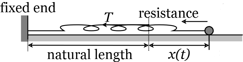
Figure 16: A spring on a table, with a mass on one end and fixed at the other end.

Solution.

The forces acting on the particle are the tension in the spring, \(T\), and the resistance, \(R\), both acting horizontally to oppose motion. By Hooke’s Law (see Example 15), the tension in the spring is \(T=k x\). The resistance is \(R=2 \beta \omega m \dot{x}\). Since both \(R\) and \(T\) act in the opposite direction to the motion, the second law of motion (Equation 106) gives

\[ \begin{equation*} \ddot{x}=-\frac{R+T}{m}=-2 \beta \omega \dot{x}-\frac{k x}{m} . \tag{124} \end{equation*} \]

Since \(\omega^{2}=k / m\), we have

\[ \begin{equation*} \ddot{x}+2 \beta \omega \dot{x}+\omega^{2} x=0 \tag{125} \end{equation*} \]

This is a homogeneous second order ODE with constant coefficients (Equation 109), so recall (Propositions 4-6) that there are three different cases, depending on the sign of \((2 \beta \omega)^{2}-4 \omega^{2}=\) \(\omega^{2}\left(\beta^{2}-1\right)\). Since \(\omega^{2}\) is positive, we just need to examine the sign of \(\beta^{2}-1\).

(a) If \(\beta=3 / 2\), Equation (125) is

\[ \begin{equation*} \ddot{x}+3 \omega \dot{x}+\omega^{2} x=0 \tag{126} \end{equation*} \]

Here, \(\beta^{2}-1=(3 / 2)^{2}-1=5 / 4>0\), so we apply Proposition 4 to give

\[ \begin{equation*} x(t)=A \exp \left(m_{+} t\right)+B \exp \left(m_{-} t\right) \tag{127} \end{equation*} \]

where (Equation 113)

\[ \begin{equation*} m_{ \pm}=\frac{-3 \omega \pm \sqrt{(3 \omega)^{2}-4 \omega^{2}}}{2}=\omega \frac{-3 \pm \sqrt{5}}{2} \tag{128} \end{equation*} \]

Hence

\[ \begin{equation*} x(t)=A \exp \left(t \omega \frac{-3+\sqrt{5}}{2}\right)+B \exp \left(t \omega \frac{-3-\sqrt{5}}{2}\right) \tag{129} \end{equation*} \]

where \(A\) and \(B\) are constants. Notice that \(\omega(-3+\sqrt{5}) / 2\) and \(\omega(-3-\sqrt{5}) / 2\) are both negative, so \(x(t) \rightarrow 0\) as \(t \rightarrow \infty\). In other words, the spring extension decays exponentially towards 0 , so the mass moves in one direction towards its equilibrium position.

(b) If \(\beta=1\), Equation (125) is

\[ \begin{equation*} \ddot{x}+2 \omega \dot{x}+\omega^{2} x=0 \tag{130} \end{equation*} \]

Here, \(\beta^{2}-1=(1)^{2}-1=0\), so we apply Proposition 5 to give

\[ \begin{equation*} x(t)=(A t+B) \exp \left(-\frac{2 \omega t}{2}\right)=(A t+B) \exp (-\omega t) \tag{131} \end{equation*} \]

where \(A\) and \(B\) are constants. Here, as \(t \rightarrow \infty,(A t+B) \exp (-\omega t) \rightarrow 0\) so at long times the mass moves exponentially towards its equilibrium location. In Figure (17), we see the four qualitative possibilities for the motion of \(x(t)\), depending on the signs of \(A\) and \(B\).

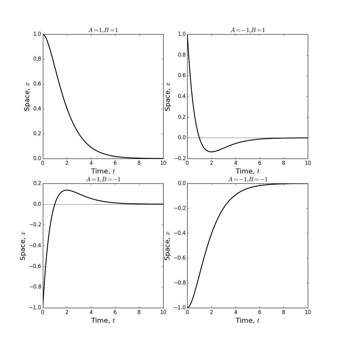
Figure 17: Examples of Equation (131) for various values of \(A\) and \(B\). Notice that for some values (e.g. \(A=B=1\) in top-left and \(A=B=-1\) in bottom-right) the mass returns monotonically to its resting location. For others (e.g. \(A=1, B=-1\) in top-right and \(A=-1, B=1\) in bottom-left) the mass moves in one direction, turns once, and then settles to its equilibrium location.

(c) If \(\beta=1 / 2\), Equation (125) is

\[ \begin{equation*} \ddot{x}+\omega \dot{x}+\omega^{2} x=0 . \tag{132} \end{equation*} \]

Here, \(\beta^{2}-1=(1 / 2)^{2}-1=-3 / 4<0\), so we apply Proposition 6 to give

\[ \begin{equation*} x(t)=\exp \left(-\frac{\omega t}{2}\right)[A \sin (q t)+B \cos (q t)] \tag{133} \end{equation*} \]

where \(A\) and \(B\) are constants and \(q=\sqrt{4 \omega^{2}-\omega^{2}} / 2=\omega \sqrt{3} / 2\). Hence

\[ \begin{equation*} x(t)=\exp \left(-\frac{\omega t}{2}\right)\left[A \sin \left(\frac{\sqrt{3}}{2} \omega t\right)+B \cos \left(\frac{\sqrt{3}}{2} \omega t\right)\right] \tag{134} \end{equation*} \]

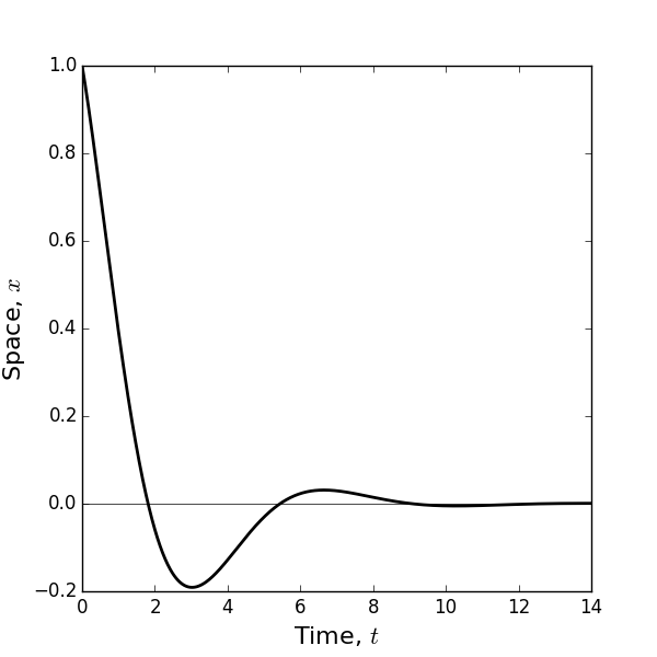
Figure 18: Example of Equation (134) with \(\omega=1, A=0, B=1\)

In this case \(x(t)\) exhibits damped oscillations. The frequency of these oscillations (i.e. the number of oscillations per unit time) is

\[ \frac{\sqrt{3}}{4 \pi} \omega \]

The sine and cosine terms cause the mass \(m\) to oscillate between a positive and negative extension, whilst the \(\exp (-\omega t / 2)\) term causes those oscillations to decrease over time. Figure 18 gives a plot of Equation (134) for \(\omega=1, A=0, B=1\).

Note

The previous example has three distinct regions, \(\beta>1, \beta=1\), and \(\beta<1\). These correspond, respectively, to the results from Propositions 4, 5, and 6. Physically, the \(\beta>1\) case is called strongly damped and the spring returns monotonically to its equilibrium state. The \(\beta<1\) case is called weakly damped and the spring undergoes damped oscillations as it returns to its equilibrium state. The \(\beta=1\) case is called critically damped and the extension of the spring may not move monotonically, but there will be at most one turning point (Figure 17).

Lecture 11 Homework exercises

Exercise 23}

A cable is used to suspend an 800 kg safe. The stiffness of the cable is \(k=20,000 \mathrm{Nm}^{-1}\) (recall that \(N\) stands for ‘Newton’ and \(1 N=1 \mathrm{kgms}^{-2}\) ).

(a) Show that, when the safe is stationary, the extension of the cable is \(a=m g / k\), where \(g\) is the acceleration due to gravity. Calculate \(a\).

(b) The safe is being lowered at \(6 \mathrm{~ms}^{-1}\) when the cable jams and suddenly stops moving. Let \(x(t)+a\) be the extension of the cable. Show that \(\ddot{x}+\omega^{2} x=0\) where \(\omega^{2}=k / m\).

(c) Solve the ODE from part (b) to show that the safe oscillates in perpetuity at a frequency of \(\omega /(2 \pi)\) and amplitude (i.e. maximum displacement from equilibrium) of \(1.2 m\).

(d) Why is this conclusion unrealistic? How might we change our model to make it more realistic?

Exercise 24

An elastic string of natural length \(2 l_{0}\) and stiffness \(k\) is stretched horizontally between two points \(A\) and \(B\) a distance \(2 l\) apart (where \(l>l_{0}\) ), in a gravity-free environment. A particle of mass \(m\) attached to the midpoint \(O\) of the string is drawn aside a small distance \(a\), where \(a<l-l_{0}\), along \(A B\) and released. Let \(x(t)\) be the location of the

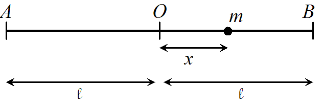
particle with respect to the origin, \(O\).

(a) Find the extensions in the segments of the string to the left and right of the mass (Hint: subtract the natural length from the stretched length).

(b) Find the tensions in each segment of the stretched string, and indicate on a diagram the directions of their actions on the particle.

(c) Use the second law of motion to find an ODE describing the motion of the mass.

(d) Solve this ODE.

Exercise 25

A particle \(P\) of mass \(m\) is tied to one end of an elastic string of natural length \(a\) and stiffness \(2 m \omega^{2}\). The other end \(B\) is attached to a point \(A\) on a fixed smooth horizontal plane. The particle is released from rest on the plane when the string is extended to a length \(2 a\). Let \(x(t)\) be the extension of the string. (a) Ignoring any friction, derive an equation governing the motion of \(x(t)\). Use this to find the speed of the particle when the string first becomes slack (i.e. when \(x(t)=0)\).

(b) Suppose now that motion is resisted by a force of \(2 m \omega(\dot{x})\). Show that \(\ddot{x}+2 \omega \dot{x}+\) \(2 \omega^{2} x=0\). Find \(x\) as a function of \(t\), and use this to find the time at which the string first becomes slack.