Lecture 12. Inhomogeneous second order ODEs

Before we go any further, let’s start with an example.

Example 18

A particle \(P\) of mass \(m\) is attached to one end of a spring of natural length \(L\) and stiffness \(k\). The other end of the spring is fixed at the point \(A\). Initially the spring hangs down vertically in equilibrium. The point \(A\) is then set in vertical motion, so that its displacement from its initial position is

\[ \begin{equation*} y(t)=D \sin (\sigma t) \tag{135} \end{equation*} \]

where \(D>0\) and \(\sigma>0\) are constants. Let \(x(t)\) be the displacement of the particle from its equilibrium position. Show that the equation of motion for the particle is

\[ \begin{equation*} \ddot{x}+\omega^{2} x=\omega^{2} D \sin (\sigma t) \tag{136} \end{equation*} \]

where \(\omega\) is a positive constant which should be determined.

Solution.

The forces acting on \(P\) are the weight, \(m g\), acting vertically downwards, and the tension, \(T\), in the spring, acting vertically upwards. In equilibrium, let the tension in the spring be \(T=T_{0}\) and the extension of the spring be \(a\). By Hooke’s Law, \(T_{0}=k a\). Since the system is in equilibrium, the vertical forces balance (Figure 19), so

\[ \begin{equation*} m g=T_{0}=k a \tag{137} \end{equation*} \]

When the system is set in motion, the distance of the spring from the fixed level is \(L+a+x\) (Figure 19), the original length of the spring, \(L+a\), plus the displacement of the particle from its original position, \(x\). Since the top of the spring is a distance \(y\) from the fixed level, the length of the spring is \(L+a+x-y\) and so the extension of the spring is \((L+a+x-y)-L=a+x-y\). By Hooke’s Law, the tension \(T\) in the spring is \(k\) times the extension, which is

\[ \begin{equation*} T=k(a+x-y) \tag{138} \end{equation*} \]

Using Newton’s Second Law in the vertical direction:

\[\begin{split} \begin{align*} m \ddot{x} & =m g-T \\ & =m g-k(a+x-y) \\ & =m g-k a-k x+k y \\ & =-k x+k y, \tag{139} \end{align*} \end{split}\]

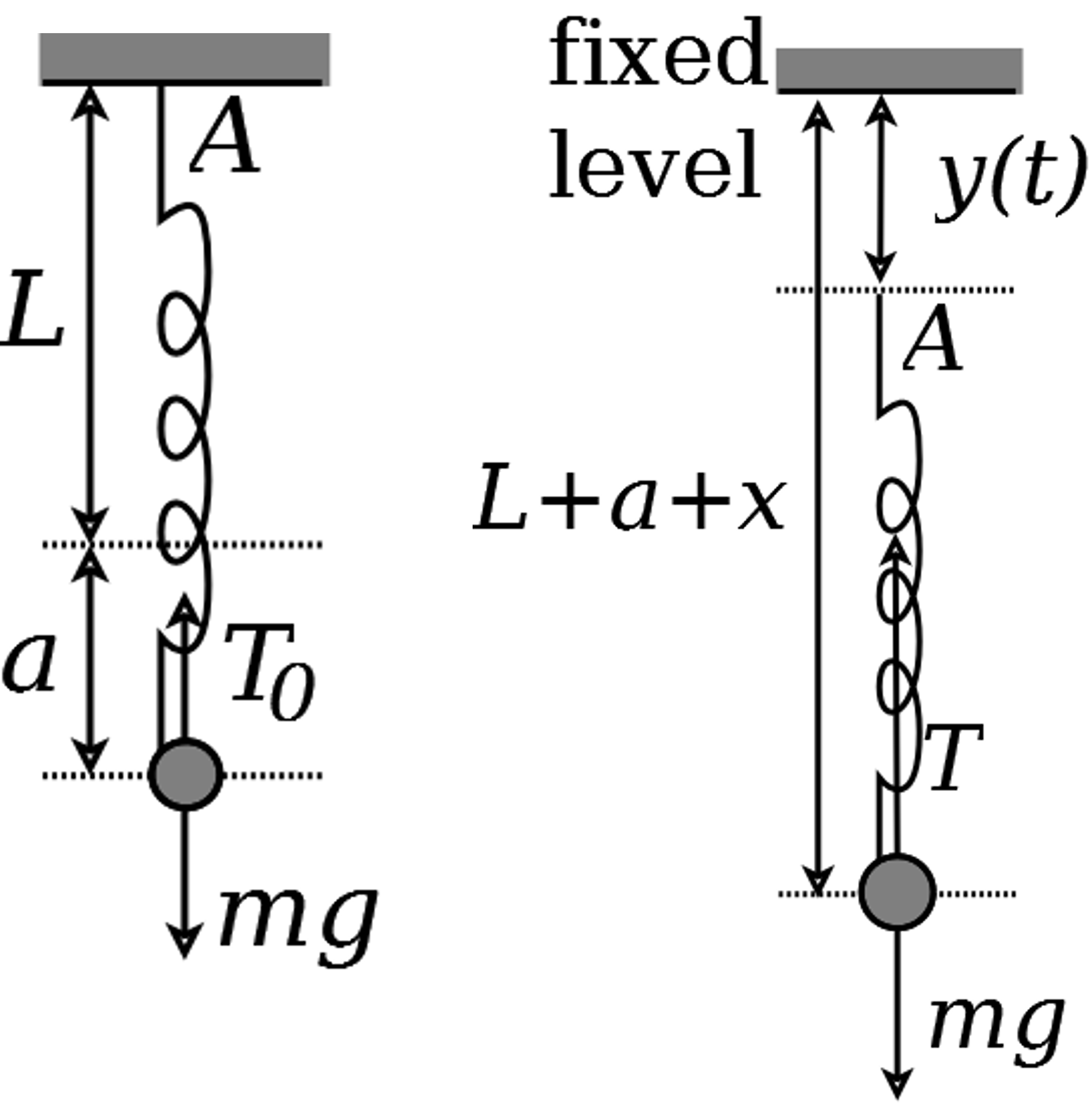
Figure 19: Left-hand plot shows the situation when the system is in equilibrium. The righthand plot is when the system is in motion.

where we have used Equation (137) in the last equality. Therefore

\[\begin{split} \begin{align*} m \ddot{x}+k x & =k y=k D \sin (\sigma t) \\ \Longrightarrow \ddot{x}+\frac{k}{m} x & =\frac{k}{m} D \sin (\sigma t), \tag{140} \end{align*} \end{split}\]

and we have

\[ \begin{equation*} \ddot{x}+\omega^{2} x=D \omega^{2} \sin (\sigma t) \tag{141} \end{equation*} \]

where \(\omega^{2}=\frac{k}{m}\), so that \(\omega=\sqrt{\frac{k}{m}}\).

Notice that the resulting ODE (Equation 141) is not in the form of Equation (109) so we cannot use our results from Propositions 4-6.

Definition 15

Definition. An equation of the following type

\[ \begin{equation*} \ddot{x}+b \dot{x}+c x=f(t) \tag{142} \end{equation*} \]

for some function \(f(t) \neq 0\) and constants \(b\) and \(c\), is called an inhomogeneous second order ODE with constant coefficients.

Notice that Equation (141) is an example of an inhomogeneous second order ODE with constant coefficients.

12.1 The method of undetermined coefficients

There is no single catch-all method for solving inhomogeneous second order ODE with constant coefficients, but there is a method that works in many cases, called the method of undetermined coefficients, as follows

1. Try to find a solution to Equation (142) of the same form as \(f(t)\), called the particular solution, \(x_{P}(t)\).

2. Solve the associated homogeneous ODE, \(\ddot{x}_{I}+b \dot{x}_{I}+c x_{I}=0\) to obtain the complementary function, \(x_{I}(t)\).

3. Then the general solution is \(x(t)=x_{I}(t)+x_{P}(t)\).

The problem with this method is that Step 1 does not always work for any function \(f(t)\). However, it usually works for polynomials, exponential functions, sine, and cosine.

Example 19

Find the general solution to Equation (141) in the case \(\sigma^{2} \neq \omega^{2}\).

Solution.

The right-hand side of Equation (141) is \(\sin (\sigma t)\), so we will try to find a solution of the form \(x(t)=A \sin (\sigma t)\). Here, \(\dot{x}(t)=A \sigma \cos (\sigma t)\) and \(\ddot{x}(t)=-A \sigma^{2} \sin (\sigma t)\). Plugging these into Equation (141) gives

\[\begin{split} \begin{align*} & A \omega^{2} \sin (\sigma t)-A \sigma^{2} \sin (\sigma t)=D \omega^{2} \sin (\sigma t) \\ \Longrightarrow & A\left(\omega^{2}-\sigma^{2}\right)=D \omega^{2} \\ \Longrightarrow & A=\frac{D \omega^{2}}{\omega^{2}-\sigma^{2}} \tag{143} \end{align*} \end{split}\]

where we have used \(\sigma^{2} \neq \omega^{2}\) in the last step. Thus the particular solution is

\[ \begin{equation*} x_{P}(t)=\frac{D \omega^{2}}{\omega^{2}-\sigma^{2}} \sin (\sigma t) \tag{144} \end{equation*} \]

Next we solve the corresponding inhomogeneous ODE

\[ \begin{equation*} \ddot{x}_{I}+\omega^{2} x_{I}=0 \tag{145} \end{equation*} \]

Using Proposition 6, we have that

\[ \begin{equation*} x_{I}(t)=B \sin (\omega t)+C \cos (\omega t) \tag{146} \end{equation*} \]

for constants \(B\) and \(C\). Then the general solution is

\[ \begin{equation*} x(t)=x_{I}(t)+x_{P}(t)=B \sin (\omega t)+C \cos (\omega t)+\frac{D \omega^{2}}{\omega^{2}-\sigma^{2}} \sin (\sigma t) \tag{147} \end{equation*} \]

The tricky thing about this method is finding a good guess for the form of the particular solution. Here’s some rules as to what you should try for certain specific functions.

1. If \(f(t)\) is a polynomial of degree \(n\), i.e. \(f(t)=a_{0}+a_{1} t+a_{2} t^{2}+\cdots+a_{n} t^{n}\), try setting \(x_{P}(t)\) to be another polynomial of degree \(n\), i.e. \(x_{P}(t)=A_{0}+A_{1} t+A_{2} t^{2}+\cdots+A_{n} t^{n}\).

2. If \(f(t)=a_{0} \exp \left(a_{1} t\right)\), try \(x_{P}(t)=A \exp \left(a_{1} t\right)\).

3. If \(f(t)=a_{0} \sin \left(a_{1} t\right)\) or \(f(t)=\cos \left(a_{1} t\right)\), try \(x_{P}(t)=A_{1} \sin \left(a_{1} t\right)+A_{2} \cos \left(a_{1} t\right)\).

4. If \(f(t)=a_{0} \sin \left(a_{1} t\right)\) and the coefficient of \(\dot{x}\) is zero, \(\operatorname{try} x_{P}(t)=A \sin \left(a_{1} t\right)\).

5. If \(f(t)=a_{0} \cos \left(a_{1} t\right)\) and the coefficient of \(\dot{x}\) is zero, try \(x_{P}(t)=A \cos \left(a_{1} t\right)\).

In the above, \(A, a_{i}\), and \(A_{i}\) (for each \(i\) ) are all constants.

Lecture 12 Homework exercises

Exercise 26

26. Find the general solution to each of the following second order ODEs

(a) \(\ddot{x}+3 \dot{x}+2 x=t\)

(b) \(\ddot{x}+2 \dot{x}-x=t^{2}\)

(c) \(\ddot{x}+2 \dot{x}+x=t^{2}+2 t+1\)

(d) \(\ddot{x}+4 \dot{x}+4 x=\sin (2 t)\)

(e) \(\ddot{x}+2 \dot{x}+4 x=\cos (3 t)\)

(f) \(\ddot{x}+\dot{x}+x=\exp (t)\)

(g) \(\ddot{x}+\dot{x}+2 x=2 t^{3}+6\)

(h) \(2 \ddot{x}+4 \dot{x}+2 x=\sin (t)+\cos (t)\)

(i) \(2 \ddot{x}+2 \dot{x}+2 x=4 \sin (4 t)\)

(j) \(3 \ddot{x}+12 \dot{x}+12 x=2 \cos (t)\)