Lecture 9. Direction fields for non-autonomous ODEs

If an ODE is non-autonomous, i.e. of the form

\[ \begin{equation*} \frac{\mathrm{d} U}{\mathrm{~d} t}=g(U, t) \tag{102} \end{equation*} \]

where the dependence of \(g\) on \(t\) is non-trivial, then you cannot construct a phase line. (Why not?) You can, however, plot a direction field. This is a plot of the directions of flow on the \((U, t)\)-plane. To illustrate what this means, we will start with an example, which will make use of some new notation.

Note

For any function of time, \(U(t)\), we sometimes use the following short hand

\[ \begin{equation*} \dot{U}=\frac{\mathrm{d} U}{\mathrm{~d} t} \tag{103} \end{equation*} \]

Example 13

Draw the direction field for a population of organisms with a seasonally fluctuating birth rate and constant intraspecific competition, given as follows

\[ \begin{equation*} \dot{U}=U\left(2-\frac{1}{2} \sin (t)-U\right) \tag{104} \end{equation*} \]

Solution.

We want to draw arrows on the \((U, t)\)-plane describing the direction of change of the solution. But the direction of change is simply the gradient of the derivative, \(\dot{U}\), and we have a formula for that in Equation (104). With this in mind, the general technique for plotting a direction field is as follows.

1. Select a point \((t, U)\).

2. At this point \((t, U)\), draw a short vector with gradient \(\dot{U}\).

3. Repeat this process for multiple values of \(t\) and \(U\) to map out the flow in \((t, U)\) space.

4. By following the directions of the arrows, the solution curves of the ODE can be determined.

It helps to start by drawing a table of values of \(\dot{U}\) for a variety of pairs of values of \((t, U)\). An example is shown in Table 8 (programming or spreadsheet software can help you construct this). Then, for each cell in this table, plot an arrow whose gradient is given by the value in the cell and whose location is given by the corresponding value of \(U\) and \(t\).

Figure 13 gives the result of this procedure (red arrows), where we have plotted a slightly wider range of values that that shown in Table 8. For example, if we look at the point on the graph where \(t=\pi\) and \(U=0.5\), we find an arrow with gradient 0.75 , highlighted in red in Table 8.

\(U \downarrow, t \rightarrow\)	0	\(\pi / 2\)	\(\pi\)	\(3 \pi / 2\)	\(2 \pi\)	\(5 \pi / 2\)	\(3 \pi\)	\(7 \pi / 2\)	\(4 \pi\)
0	0	0	0	0	0	0	0	0	0
0.5	0.75	0.5	0.75	1	0.75	0.5	0.75	1	0.75
1	1	0.5	1	1.5	1	0.5	1	1.5	1
1.5	0.75	0	0.75	1.5	0.75	0	0.75	1.5	0.75
2	0	-1	0	1	0	-1	0	1	0
2.5	-1.25	-2.5	-1.25	0	-1.25	-2.5	-1.25	0	-1.25
3	-3	-4.5	-3	-1.5	-3	-4.5	-3	-1.5	-3
3.5	-5.25	-7	-5.25	-3.5	-5.25	-7	-5.25	-3.5	-5.25
4	-8	-10	-8	-6	-8	-10	-8	-6	-8

Table 8: The first row gives values of \(t\) and the first column gives values of \(U\). The other cells show values of \(\dot{U}\) for the corresponding values of \(U\) and \(t\), as determined by Equation (104).

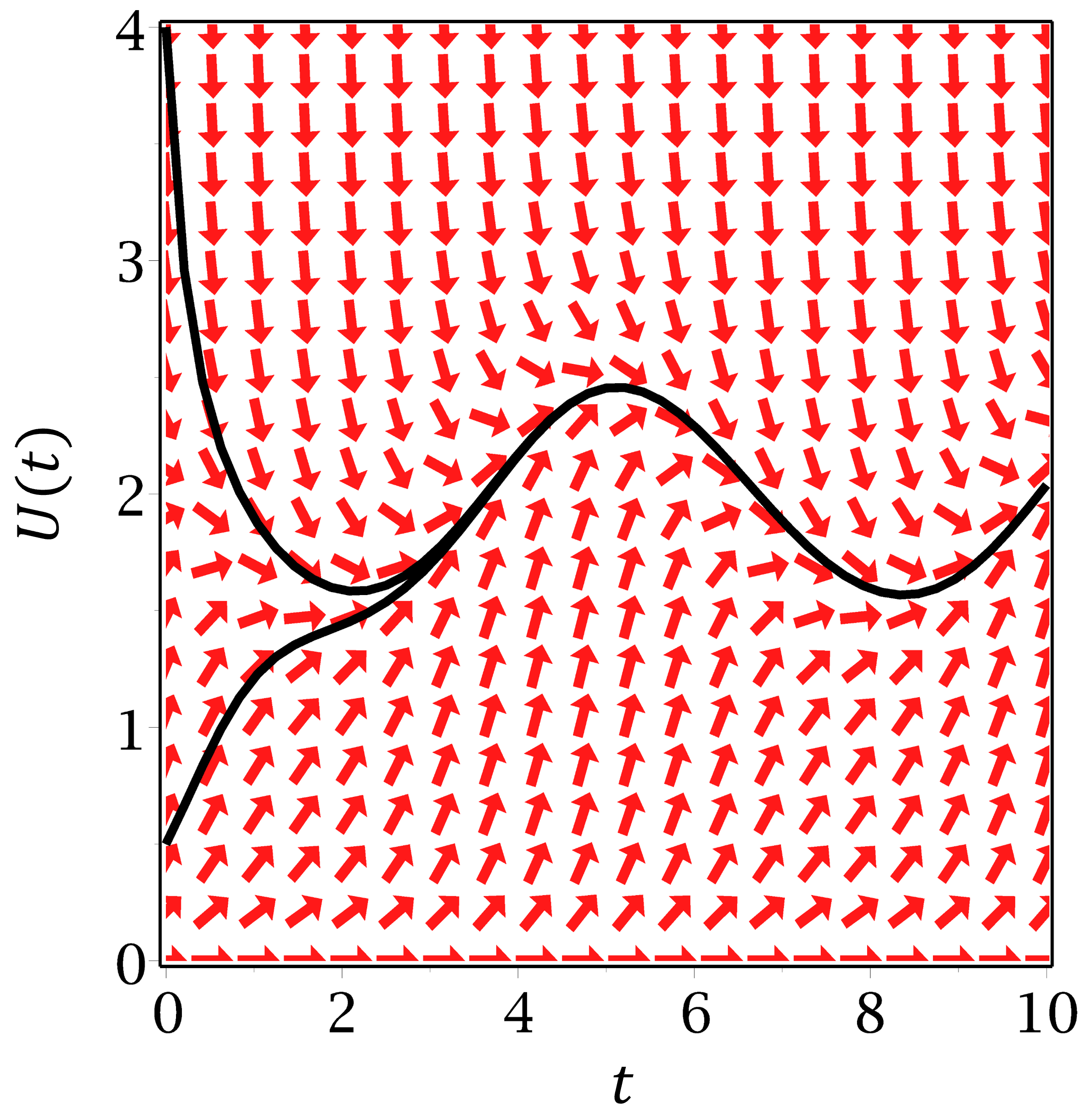
Figure 13: Direction field for Equation (104).

Figure 13 also shows the solution to Equation (104) for two different initial conditions: \(U(0)=4\), given by the top curve, and \(U(0)=1 / 2\), given by the bottom curve. These are not algebraic expressions, but rather they are graphical solutions, showing how \(U\) changes over time. Nonetheless, they are still solutions, and valuable for analysing ODEs.

Example 14

Suppose we have a population of animals living in an environment that is being slowly degraded over time (e.g. by climate change or deforestation). We can model this environmental degradation as a decline of carrying capacity: as the environment degrades, it is able to sustain less individuals. A simple model of this is as follows

\[ \begin{equation*} \dot{U}=r U\left(1-\frac{U}{K \exp (-\mu t)}\right) \tag{105} \end{equation*} \]

Plot the direction field in the case \(r=K=\mu=1\) for \(0 \leq U \leq 2\) and \(0 \leq t \leq 3\). What do you think will happen to \(U(t)\) as \(t \rightarrow \infty\) ? Why?

Solution.

Values of \(\dot{U}\) for various \(0 \leq U \leq 2\) and \(0 \leq t \leq 3\) are given in Table 9. The resulting direction field is shown in Figure 14. If we start at any initial location \(U(0)\), we see that the trajectory seems to be tending to 0 , so the animals die out. This is because the carrying capacity is \(\exp (-t)\), which tends to zero over time, i.e. the size of population that the environment can sustain decreases to zero over time.

\(U \downarrow, t \rightarrow\)	0	0.5	1	1.5	2	2.5	3
0	0.0	0.0	0.0	0.0	0.0	0.0	0.0
0.25	0.2	0.1	0.1	0.0	-0.2	-0.5	-1.0
0.5	0.3	0.1	-0.2	-0.6	-1.3	-2.5	-4.5
0.75	0.2	-0.2	-0.8	-1.8	-3.4	-6.1	-10.5
1	0.0	-0.6	-1.7	-3.5	-6.4	-11.2	-19.1
1.25	-0.3	-1.3	-3.0	-5.8	-10.3	-17.8	-30.1
1.5	-0.8	-2.2	-4.6	-8.6	-15.1	-25.9	-43.7
1.75	-1.3	-3.3	-6.6	-12.0	-20.9	-35.6	-59.8
2	-2.0	-4.6	-8.9	-15.9	-27.6	-46.7	-78.3

Table 9: The first row gives values of \(t\) and the first column gives values of \(U\). The other cells show values of \(\dot{U}\) for the corresponding values of \(U\) and \(t\), as determined by Equation (104).

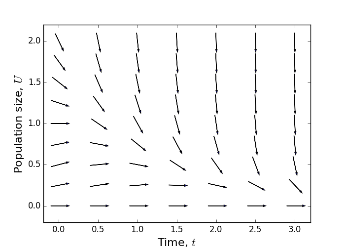
Figure 14: Direction field for Equation (105).

Lecture 9 Homework exercises

Exercise 19

For each of the following ODEs, draw direction fields. Add some example solution trajectories to the plots.

(a) \(\dot{U}=U(1-U)\)

(b) \(\dot{U}=t \sin (U)\)

(c) \(\dot{U}=U \sin (t)\)

(d) \(\dot{U}=U^{3}-6 U^{2}+11 U-6\)