Lecture 3. Cycles, period-doubling, and chaos

If you did Exercise 3 from Lecture 2 for your homework, you will have seen some interesting patterns emerge from the logistic model. This lecture, we are going to study the wealth of such patterns and learn how to categorise them. We will work with a version of the logistic map where \(K=1\). You can thus think of \(U(t)\) as being given in units of thousands of organisms (or millions of organisms) so that \(K=1\) means that the carrying capacity of the environment is a thousand (or a million) organisms. We will also talk about an ‘organism’ rather than a ‘rabbit’ in this lecture, since there is nothing mathematically special about rabbits (just that they are fluffy and cute and breed a lot). This also gives you the chance to picture your favourite animal, plant, archaea, or whatever, as your study organism.

So, just to be clear, the study equation for this lecture will be

\[ \begin{equation*} U(t+1)=U(t)+r U(t)[1-U(t)] \tag{15} \end{equation*} \]

which is just Equation (7) with \(K=1\). Let’s start off with \(r=1\) and \(U(0)=0.1\). As in the previous lecture, we can calculate a table of values, see Table 3.

Time, \(t\) years	0	1	2	3	4	5	6	7	8	9	10
Population size, \(U(t)\)	0.1	0.19	0.34	0.57	0.81	0.97	1.0	1.0	1.0	1.0	1.0

Table 3: Change in population size over time, using the model in Equation (15) with \(r=1\) and \(U(0)=0.1\).

Very often in modelling, when we start dealing with real numerics, the calculations can quickly become a bit of a handful. We therefore regulary start plugging numbers into some sort of numerical software to make the calculations easier. There are different levels of difficulty for achieving this, from simply repeatedly plugging numbers into a calculator, to using a spreadsheet like Excel with formulae in, to using programming languages like Python or R. While my predecessor on this course provided Excel spreadsheets - probably familiar to more of you and so in a sense more accessible - I have chosen to provide you with Python code. Much of what I provide will be set-up so that all you have to do is click some buttons, but since programming is an increasingly central pillar of mathematical modelling, I think it is useful for you to get used to looking at some code.

For this first example I have provided some code where you can simply move a slider to change the value of \(r\) in the model. You are very welcome to reveal the code behind this to see what is going on behind the curtain. There is also sample code at the end of this lecture which you can copy and paste into Google Colab yourself.

Time, \(t\) years	0	1	2	3	4	5	6	7	8	9	10
Population size, \(U(t)\)	0.10	0.24	0.50	0.88	1.04	0.98	1.01	0.99	1.0	1.0	1.0

Table 4: Change in population size over time, using the model in Equation (15) with \(r=1.5\) and \(U(0)=0.1\).

Let’s examine what happens to the logistic model as we increase \(r\). Table 4 shows the case when \(r=1.5\). Like the \(r=1\) case, \(U(t)\) starts by increasing over the first few time steps. At \(t=4\), however, \(U(t)\) overshoots the carrying capacity, as \(U(4)=1.04\). It then decreases in the next step, to \(U(5)=0.98\). It then goes back up, but to a smaller value of \(U(6)=1.01\), and we see these oscillations gradually die down so that the solution reaches a steady state. Figure 6a shows this solution up to \(t=50\), and there we can see the solutions settling down quite clearly to \(U(t)=1\).

Time, \(t\) years	0	1	2	3	4	5	6	7	8	9	10
Population size, \(U(t)\)	0.10	0.30	0.76	1.16	0.75	1.16	0.75	1.16	0.75	1.16	0.75

Table 5: Change in population size over time, using the model in Equation (15) with \(r=2.2\) and \(U(0)=0.1\).

For \(r=2.2\), we see another phenomenon. The value of \(U(t)\) increases at the start, but then, from about \(t=3\) onwards, it appears to oscillate between 0.75 and 1.16. This oscillation continues if we extend the sequence for longer (Figure 6 b ). We can actually find the precise values that the solution oscillates between. Let’s call them \(A\) and \(B\). Then, plugging \(U(t+1)=B\) and \(U(t)=A\) into Equation (15), we have

\[ \begin{equation*} B=A+r A(1-A) \tag{16} \end{equation*} \]

Now we plug \(U(t+1)=A\) and \(U(t)=B\) into Equation (15), to give

\[ \begin{equation*} A=B+r B(1-B) \tag{17} \end{equation*} \]

Plugging Equation (17) into Equation (16) gives

\[ \begin{equation*} B=B+r B(1-B)+r[B+r B(1-B)][1-B-r B(1-B)] \tag{18} \end{equation*} \]

Equation (18) has an exact solution. It’s a long task to figure this out by hand, so instead we can just go on the www.wolframalpha.com website and type in our equation.

It then tells us that

\[\begin{equation*} B=\frac{r+2 \pm \sqrt{r^{2}-4}}{2 r} \tag{19} \end{equation*}\]

Notice a few things. First, \(A\) has the same solutions a \(B\). This can be seen simply by swaping \(A\) and \(B\) around in the above argument. Second, \(B\) is only defined when \(r^{2}>4\), i.e. \(r>2\) (for those who know about imaginary numbers, \(B\) must be real; for those who don’t, just ignore this parenthetic comment). Third, if we put in \(r=2.2\), we get \(B=0.746247,1.16284\), to six significant figures, which agrees with what we observed in Table 5.

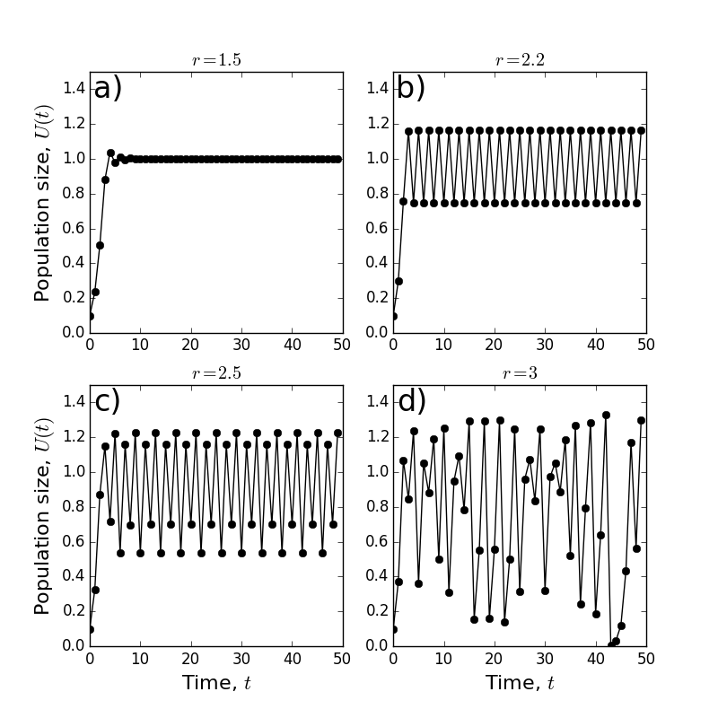
Figure 6: Evolution of the logistic model from Equation (15), for (a) \(r=1.5\), (b) \(r=2.2\), (c) \(r=2.5\), (d) \(r=3\).

This example shows that, even though a difference equation may admit steady states, it may never reach them. Equation (15) has steady states of 0 and 1 for any \(r\) (see Example 4), but it does not reach them if \(r=2.2\) and \(U(0)=0.1\).

Time, \(t\) years	0	1	2	3	4	5	6	7	8	9	10
Population size, \(U(t)\)	0.10	0.33	0.87	1.15	0.72	1.22	0.54	1.16	0.70	1.22	0.54

Table 6: Change in population size over time, using the model in Equation (15) with \(r=2.5\) and \(U(0)=0.1\).

Table 6 shows the case where \(r=2.5\). Here, after going up until \(t=3\), \(U(t)\) begins to oscillate up and down. However, unlike the \(r=2.2\) example, it does not settle on a pair of values. Continuing the sequence for more time, we see that the system oscillates between four values: \(1.16,0.70,1.22\), and 0.54 (see Figure 6 c ). In principle, one can calculate these by solving the following simultaneously

\[\begin{split} \begin{align*} & B=A+r A(1-A) \\ & C=B+r B(1-B) \\ & D=C+r C(1-C) \\ & A=D+r D(1-D) \tag{20} \end{align*} \end{split}\]

but it is a rather lengthy calculation, so I won’t suffer you with it. Instead, I’ll give you a definition.

Definition 3

Definition. Let \(U(t)\) be a sequence of real numbers defined for each non-negative integer, \(t\). If there are non-negative integers \(T\) and \(\tau\) such that \(U(t+\tau)=U(t)\) for each \(t>T\) (and there is no smaller value of \(\tau\) with this property) then we say that \(U(t)\) settles to a period \(\tau\) oscillation at long times.

Therefore the \(r=2.2\) case settles to a period 2 oscillation (at long times) and the \(r=2.5\) case settles to a period 4 oscillation. We say that there is a period doubling bifurcation between \(r=2.2\) and \(r=2.5\).

Time, \(t\) years	0	1	2	3	4	5	6	7	8	9	10
Population size, \(U(t)\)	0.10	0.37	1.07	0.85	1.24	0.36	1.05	0.88	1.19	0.50	1.25

Table 7: Change in population size over time, using the model in Equation (15) with \(r=3\) and \(U(0)=0.1\).

Now let’s look at \(r=3\) (Table 7, Figure 6d). What in the heck is going on there? Well, mathematicians call this ‘chaos’ and perhaps you can see why! There is no clear pattern to the sequence \(U(t)\) any more. The notion of chaos can be formalised and quantified in various ways, but this is way too advanced for the present module. So we will stop our analysis of Equation (15) here, just to say that if you are interested, search for ‘period doubling route to chaos’ and read more about it. The book ‘Chaos’ by James Gleick is also a great, non-technical introduction to this fascinating subject.

Before we finish, though, we should go back to the original scientific question, which was about predicting the change in size of a population of organisms. The answer depends upon \(r\). For small \(r\), e.g. \(r=1\), the population will grow monotonically, approaching a steady state as \(t \rightarrow \infty\). For slightly larger \(r\), e.g. \(r=1.5\), the population grows initially, before oscillating around the steady state. However, these oscillations dampen over time and the population settles to steady state (Figure 6a). If \(r\) is larger still, e.g. \(r=2.2\) or \(r=2.5\), the population size never settles but will oscillate in perpetuity in a predictive fashion (Figure 6b,c). If \(r\) becomes even larger, there are no longer clear oscillations, but just a ‘chaotic’ jumping between different values. If we are in such a situation in real life, it becomes incredible hard both to fit data to the model and to predict the future.

Lecture 3 Homework exercises

Exercises

If you did not use any software to answer Exercises 3 and 4 from Lecture 2, revisit them by using the code provided, which should enable you to repeat your analysis up to higher values of \(t\).

Otherwise, catch up with any exercises from Lecture 2 that you have not yet completed.

#First we get Python to import any libraries it needs
import numpy as np
import matplotlib.pyplot as plt

#Next we define a 'function' to compute the next value
def discrete_logistic(x,r):
    #NOTE: notice the indent - this is very important for Python and must be kept
    x1=x+r*x*(1-x)
    return x1

r=1
x0=0.1  #Initial condition for our population
xstore=[x0] #Store all the population nimbers

#Run the model by looping through all the time points
for t in range(1,41):
    xstore.append(discrete_logistic(xstore[-1],r))

#Code to plot the output
#The first two lines set the figure and font size
plt.rcParams['figure.figsize'] = [8, 4]#
plt.rcParams.update({'font.size': 16})

# The next lines plot the output and give some labels
plt.plot(xstore,'b', marker = 'o')
plt.xlabel('Time')
plt.ylabel('Numbers')