Lecture 13. Modelling oscillations with second order ODEs: a worked example

In the last three lectures, we introduced both homogeneous and inhomogeneous ODEs, showing how they can be used to model oscillatory motion. Here we will work through a single example that encompasses the various cases we have looked at: undamped motion, damped motion, and forced motion.

Example 20

A particle \(P\) of mass \(m\) is tied to one end of an elastic string of natural length \(a\) and stiffness \(2 m \omega^{2}\). The other end \(B\) is attached to a point \(A\) on a fixed smooth horizontal plane. The particle is released from rest on the plane when the string is extended to a length \(2 a\).

(a) Undamped motion. If the subsequent motion is unresisted, find an expression for extension, \(x(t)\), of the string at time \(t\).

(b) Damped motion. Suppose now that the subsequent motion is resisted by a force \(2 m \omega\) times the speed. Show that

\[ \begin{equation*} \ddot{x}+2 \omega \dot{x}+2 \omega^{2} x=0 \quad(x \geq 0) \tag{148} \end{equation*} \]

Find \(x\) as a function of \(t\), and show that the speed of the particle at the moment the string becomes slack is

\[ \begin{equation*} \omega a \sqrt{2} e^{-\frac{3 \pi}{4}} \tag{149} \end{equation*} \]

(c) Forced motion. Finally, suppose that the motion is resisted as described in part (b), but, instead of the other end of the string being fixed, it is forced to oscillate so that the distance of \(B\) from \(A\) at time \(t\) is

\[ \begin{equation*} y(t)=a[2 \sin (\omega t)-\cos (\omega t)] . \tag{150} \end{equation*} \]

In this case, show that the equation of motion is

\[ \begin{equation*} \ddot{x}+2 \omega \dot{x}+2 \omega^{2} x=-5 a \omega^{2} \cos (\omega t) \tag{151} \end{equation*} \]

and find \(x\) as a function of \(t\).

Solution.

(a) By Hooke’s law, the tension in the string when it is extended a distance \(x\) is \(T=2 m \omega^{2} x\). Since \(T\) is the only force acting on the mass (Figure 20), the second law of motion (Equation 106) says that

\[\begin{split} \begin{align*} & m \ddot{x}=-T=-2 m \omega^{2} x, \\ \Longrightarrow & \ddot{x}+2 \omega^{2} x=0 \tag{152} \end{align*} \end{split}\]

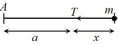
Figure 20: Forces acting on the string in Example 20a.

By Proposition 6, the general solution to Equation (152) is

\[ \begin{equation*} x(t)=A \cos (\sqrt{2} \omega t)+B \sin (\sqrt{2} \omega t) \tag{153} \end{equation*} \]

where \(A\) and \(B\) are arbitrary constants. Since the string is initially stretched to a length \(2 a\), the initial extension is \(a\), i.e. \(x(0)=a\). This means that \(A=a\) so

\[ \begin{equation*} x(t)=a \cos (\sqrt{2} \omega t)+B \sin (\sqrt{2} \omega t) \tag{154} \end{equation*} \]

Since the particle starts at rest, we have \(\dot{x}(0)=0\). To apply this condition, we need to differentiate \(x(t)\) to give

\[ \begin{equation*} \dot{x}(t)=-a \sqrt{2} \omega \sin (\sqrt{2} \omega t)+B \sqrt{2} \omega \cos (\sqrt{2} \omega t) \text {. } \tag{155} \end{equation*} \]

Plugging in \(t=0\) and \(\dot{x}(0)=0\) gives \(B \sqrt{2} \omega=0\) so that \(B=0\). Therefore

\[ \begin{equation*} x(t)=a \cos (\sqrt{2} \omega t) \tag{156} \end{equation*} \]

(b) In this case, the forces are shown in the diagram below

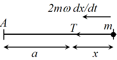
Using Newton’s second law, the equation of motion is

\[\begin{split} \begin{align*} & m \ddot{x}=-2 m \omega \dot{x}-T=-2 m \omega \dot{x}-2 m \omega^{2} x, \\ \Longrightarrow & \ddot{x}+2 \omega \dot{x}+2 \omega^{2} x=0 . \tag{157} \end{align*} \end{split}\]

We can then apply Proposition (6) to give

\[ \begin{equation*} x(t)=e^{-\omega t}[A \cos (\omega t)+B \sin (\omega t)] \tag{158} \end{equation*} \]

where \(A\) and \(B\) are arbitrary constants. Using the initial condition \(x=a\) when \(t=0\) gives \(A=a\), so that

\[ \begin{equation*} x(t)=e^{-\omega t}[a \cos (\omega t)+B \sin (\omega t)] \tag{159} \end{equation*} \]

As in part (a), since the particle starts at rest, we have \(\dot{x}(0)=0\). To apply this condition, we need to differentiate \(x(t)\) to give

\[ \begin{equation*} \dot{x}(t)=-\omega e^{-\omega t}[a \cos (\omega t)+B \sin (\omega t)]+e^{-\omega t}[-a \omega \sin (\omega t)+B \omega \cos (\omega t)] . \tag{160} \end{equation*} \]

Plugging in \(t=0\) and \(\dot{x}=0\) gives \(0=-a \omega+B \omega\) so that \(B=a\). The solution is then

\[ \begin{equation*} x(t)=a e^{-\omega t}[\cos (\omega t)+\sin (\omega t)] \tag{161} \end{equation*} \]

The string becomes slack when \(x=0\), which is when \(\cos (\omega t)+\sin (\omega t)=0\), i.e. \(\tan (\omega t)=-1\). The lowest \(t>0\) for which \(\tan (\omega t)=-1\) is when \(\omega t=\frac{3 \pi}{4}\) so \(t=\frac{3 \pi}{4 \omega}\). Using Equation (160), we have

\[\begin{split} \begin{array}{r} \dot{x}\left(\frac{3 \pi}{4 \omega}\right)=a e^{-\frac{3 \pi}{4}}\left[-\omega \sin \left(\frac{3 \pi}{4}\right)+\omega \cos \left(\frac{3 \pi}{4}\right)\right] \\ \quad=a e^{-\frac{3 \pi}{4}}\left[-\omega \frac{\sqrt{2}}{2}-\omega \frac{\sqrt{2}}{2}\right]=-a e^{-\frac{3 \pi}{4}} \omega \sqrt{2} \end{array} \end{split}\]

(If you didn’t know that \(\sin (3 \pi / 4)=\sqrt{2} / 2\) and \(\cos (3 \pi / 4)=-\sqrt{2} / 2\), now is the time to make sure you do!) Therefore the speed of the particle is

\[ \begin{equation*} \left|\dot{x}\left(\frac{3 \pi}{4 \omega}\right)\right|=a \omega \sqrt{2} e^{-\frac{3 \pi}{4}} \tag{163} \end{equation*} \]

(c) In this case, the force diagram is

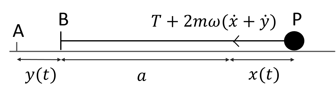
The displacement of the particle from the fixed point \(A\) is now \(x+a+y\). Therefore the velocity of the particle is \(\dot{x}+\dot{y}\) and the acceleration of the particle is \(\ddot{x}+\ddot{y}\). Using Newton’s second law, the equation of motion is

\[\begin{split} \begin{align*} & m(\ddot{x}+\ddot{y})=-2 m \omega(\dot{x}+\dot{y})-2 m \omega^{2} x \\ \Longrightarrow & \ddot{x}+2 \omega \dot{x}+2 \omega^{2} x=-\ddot{y}-2 \omega \dot{y} \tag{164} \end{align*} \end{split}\]

In the question, we are given that

\[ \begin{equation*} y(t)=a[2 \sin (\omega t)-\cos (\omega t)] \tag{165} \end{equation*} \]

Therefore

\[\begin{split} \begin{align*} & \dot{y}(t)=a \omega[2 \cos (\omega t)+\sin (\omega t)] \tag{166}\\ & \ddot{y}(t)=a \omega^{2}[-2 \sin (\omega t)+\cos (\omega t)] \tag{167} \end{align*} \end{split}\]

and therefore Equation (164) becomes

\[\begin{split} \begin{align*} \ddot{x}+2 \omega \dot{x}+2 \omega^{2} x & =a \omega^{2}[2 \sin (\omega t)-\cos (\omega t)-4 \cos (\omega t)-2 \sin (\omega t)] \\ & =-5 a \omega^{2} \cos (\omega t) \tag{168} \end{align*} \end{split}\]

The complementary function for this differential equation has already been found in the previous part (Equation 161), so we only need to find a particular solution. For this, try

\[ \begin{equation*} x_{P}(t)=p \cos (\omega t)+q \sin (\omega t) \tag{169} \end{equation*} \]

where \(p\) and \(q\) are constants to be determined. Then

\[\begin{split} \begin{align*} & \dot{x}_{P}(t)=-p \omega \sin (\omega t)+q \omega \cos (\omega t) \tag{170}\\ & \ddot{x}_{P}(t)=-p \omega^{2} \cos (\omega t)-q \omega^{2} \sin (\omega t) . \tag{171} \end{align*} \end{split}\]

Substituting Equations (170-171) into Equation (168) gives

\[\begin{split} \begin{align*} -p \omega^{2} \cos (\omega t)-q \omega^{2} \sin (\omega t)+2 \omega[-p \omega \sin (\omega t)+q \omega \cos (\omega t)] & +2 \omega^{2}[p \cos (\omega t)+q \sin (\omega t)] \\ & =-5 a \omega^{2} \cos (\omega t) \tag{172} \end{align*} \end{split}\]

We now equate the coefficients of \(\cos (\omega t)\) and \(\sin (\omega t)\) on either side of the equation, giving the following two equations for \(p\) and \(q\)

\[\begin{split} \begin{align*} & -p \omega^{2}+2 q \omega^{2}+2 p \omega^{2}=-5 a \omega^{2} \\ & -q \omega^{2}-2 p \omega^{2}+2 q \omega^{2}=0 \tag{173} \end{align*} \end{split}\]

which simplify to \(p+2 q=-5 a\) and \(-2 p+q=0\). From the second of these equations, \(q=2 p\). Substituting this into the first equation gives \(5 p=-5 a\), so \(p=-a\), and so \(q=-2 a\).

Plugging these values for \(p\) and \(q\) into Equation 169, we obtain the following particular solution of the differential equation

\[ \begin{equation*} x_{P}(t)=-a[\cos (\omega t)+2 \sin (\omega t)] \tag{174} \end{equation*} \]

The general solution is found by adding \(x_{P}(t)\) to the right-hand side of the complementary function (Equation 161). This gives

\[ \begin{equation*} x(t)=x_{P}(t)+x_{I}(t)=a e^{-\omega t}[\cos (\omega t)+\sin (\omega t)]-a[\cos (\omega t)+2 \sin (\omega t)] . \tag{175} \end{equation*} \]

Lecture 13 Homework exercises

Exercise 27

Repeat Example 20c, but instead of \(y(t)=a[2 \sin (\omega t)-\cos (\omega t)]\), as in Equation (150), use the following

(a) \(y(t)=a \sin (\omega t)\)

(b) \(y(t)=a[\sin (\omega t)+\cos (\omega t)]\)